Prediction of coloration in spatial audio systems
Assume we have a live performance of three singers at different positions. Using spatial audio systems like Wave Field Synthesis we might be able to synthesize their corresponding sound field in a way that we are convinced they are exactly at those positions they were during their actual performance. But what we most probably not be able to synthesize correctly is the timbre of those singers and listeners will perceive a coloration compared to the original performance.
We did different listening tests where we investigated the amount of coloration listeners perceive in different Wave Field Synthesis systems with a varying number of loudspeakers and the distance between adjacent loudspeakers.
The Two!Ears model has a ColorationKS that is able to predict the amount of coloration compared to a reference. The model learns this reference on the fly by choosing the first audio input it gets after the start of the Blackboard system.
In the following we show you how to get the results for listening tests from our database and how to use the Two!Ears model to predict the data.
Getting listening test data
The Database contains lots of so called human labels, which are varying data, that all comes from listening tests and has somehow human behavior as input. This can be in the form of direct rating of specific attributes like localisation or coloration, but also indirect input like measurements of the head movements of the listeners during their tasks.
In the following we are interested in modelling the results for the coloration experiment performed with WFS, which is described in 2015-10-01: Coloration of a point source in Wave Field Synthesis revisited. We did the experiment for different listening positions, loudspeaker arrays, and audio source materials. In this example, we will focus on the central listening position, a circular loudspeaker array, and speech as source material.
First, we will get the source signal and the listening test results and corresponding BRS files:
sourceMaterial = audioread(db.getFile('experiments/2015-10-01_wfs_coloration/stimuli/speech.wav'));
humanLabels = readHumanLabels(['experiments/2015-10-01_wfs_coloration/analysis/data_mean/', ...
                'coloration_wfs_circular_center_speech.csv']);
You could listen to the audio source material with and have a look at the results from the listening test:
>> sound(sourceMaterial, 48000);
>> humanLabels

humanLabels =

    'experiments/2015-10-01_wfs_coloration/brs/wfs_...'    [-0.9118]    [0.0641]
    'experiments/2015-10-01_wfs_coloration/brs/wfs_...'    [-0.4889]    [0.1948]
    'experiments/2015-10-01_wfs_coloration/brs/wfs_...'    [-0.0558]    [0.2083]
    'experiments/2015-10-01_wfs_coloration/brs/wfs_...'    [-0.1402]    [0.2176]
    'experiments/2015-10-01_wfs_coloration/brs/wfs_...'    [-0.4882]    [0.1478]
    'experiments/2015-10-01_wfs_coloration/brs/wfs_...'    [-0.4136]    [0.2215]
    'experiments/2015-10-01_wfs_coloration/brs/wfs_...'    [-0.7068]    [0.1239]
    'experiments/2015-10-01_wfs_coloration/brs/wfs_...'    [-0.8621]    [0.0824]
    'experiments/2015-10-01_wfs_coloration/brs/wfs_...'    [-0.7680]    [0.1422]
    'experiments/2015-10-01_wfs_coloration/brs/wfs_...'    [ 0.6618]    [0.1643]
The first column of humanLabels lists the corresponding BRS file used
during the experiment, the second column the median coloration rating – ranging
from -1 for not colored to 1 for strongly colored – and the third column
the confidence interval of the ratings.
Setting up the Binaural Simulator
The Binaural simulator is then setup with the BRS renderer:
sim = simulator.SimulatorConvexRoom();
set(sim, ...
    'BlockSize',            48000, ...
    'SampleRate',           48000, ...
    'NumberOfThreads',      3, ...
    'LengthOfSimulation',   5, ...
    'Renderer',             @ssr_brs, ...
    'Verbose',              false, ...
    'Sources',              {simulator.source.Point()}, ...
    'Sinks',                simulator.AudioSink(2) ...
    );
set(sim.Sinks, ...
    'Name',                 'Head', ...
    'UnitX',                [ 0.00 -1.00  0.00]', ...
    'UnitZ',                [ 0.00  0.00  1.00]', ...
    'Position',             [ 0.00  0.00  1.75]' ...
    );
set(sim.Sources{1}, ...
    'AudioBuffer',          simulator.buffer.FIFO(1) ...
    );
% First BRS entry corresponds to the reference condition
sim.Sources{1}.IRDataset = simulator.DirectionalIR(humanLabels{1,1});
sim.Sources{1}.setData(sourceMaterial);
sim.Init = true;
Estimating the coloration with the Blackboard
Now the audio part is prepared and we only have to setup the Blackboard system and estimate a coloration value for every condition with the ColorationKS:
% === Estimate reference
bbs = BlackboardSystem(0);
bbs.setRobotConnect(sim);
bbs.setDataConnect('AuditoryFrontEndKS');
ColorationKS = bbs.createKS('ColorationKS', {'speech'});
bbs.blackboardMonitor.bind({bbs.scheduler}, {bbs.dataConnect}, 'replaceOld', ...
                           'AgendaEmpty' );
bbs.blackboardMonitor.bind({bbs.dataConnect}, {ColorationKS}, 'replaceOld' );
bbs.run(); % The ColorationKS runs automatically until the end of the signal
sim.ShutDown = true;

% === Estimate coloration for every conditions
for jj = 1:size(humanLabels,1)
    sim.Sources{1}.IRDataset = simulator.DirectionalIR(humanLabels{jj,1});
    sim.Sources{1}.setData(sourceMaterial);
    sim.Init = true;
    bbs.run()
    prediction(jj) = ...
        bbs.blackboard.getLastData('colorationHypotheses').data.differenceValue;
    sim.ShutDown = true;
end
The model returned a coloration estimation for every condition in the range of
0..1 where 0 means no coloration and 1 strongly colored:
>> prediction

prediction =

    0.0007    0.1907    0.4678    0.2018    0.3461    0.2382    0.2580    0.1937

    0.1891    1.3325
The anchor condition, which is the very last entry, was rated to be even more degraded than 1. This reflects that the model is more optimised for comb-filter like spectra at the moment and not for strongly low- or high-passed signals.
Verify the results
Now, its time to compare the results with the ones from the listening test. Note, that the listening test ratings were in the range -1..1 and we have to transfer them to 0..1:
figure; hold on;
% Plot listening test results as points with errorbars
errorbar(([humanLabels{:,2}]+1)./2, [humanLabels{:,3}]./2, 'og');
% Plot model predictions as line
plot(prediction, '-g');
axis([0 11 0 1]);
xlabel('System');
ylabel('Coloration');
set(gca, 'XTick', [1:10]);
set(gca, 'XTickLabel', ...
    {'ref', 'st.', '67cm', '34cm', '17cm', '8cm', '4cm', '2cm', '1cm', 'anch.'});
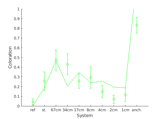
Fig. 78 Median of coloration ratings (points) together with confidence intervals and model prediction (line). The centimeter values describe the inter-loudspeaker distances for the investigated WFS systems.
To see the prediction results for all listening test data, go to the
examples/qoe_coloration folder. There you will find the following functions
that you can run, and that will pop up with a figure showing the results at the
end:
colorationWfsCircularCenter
colorationWfsCircularOffcenter
colorationWfsLinearCenter
colorationWfsLinearOffcenter