Adaptation (adaptationProc.m)
This processor corresponds to the adaptive response of the auditory nerve fibers, in which abrupt changes in the input result in emphasised overshoots followed by gradual decay to compressed steady-state level [Smith1977], [Smith1983]. The function is adopted from the Auditory Modeling Toolbox [Soendergaard2013]. The adaptation stage is modelled as a chain of five feedback loops in series. Each of the loops consists of a low-pass filter with its own time constant, and a division operator [Pueschel1988], [Dau1996], [Dau1997a]. At each stage, the input is divided by its low-pass filtered version. The time constant affects the charging / releasing state of the filter output at a given moment, and thus affects the amount of attenuation caused by the division. This implementation realises the characteristics of the process that input variations which are rapid compared to the time constants are linearly transformed, whereas stationary input signals go through logarithmic compression.
| Parameter | Default | Description |
|---|---|---|
adpt_lim |
10 |
Overshoot limiting ratio |
adpt_mindB |
0 |
Lowest audible threshold of the signal in dB SPL |
adpt_tau |
[0.005
0.050
0.129
0.253
0.500] |
Time constants of feedback loops |
adpt_model |
''(empty) |
Implementation model
can be used instead of the above three parameters (See Table 22) |
The adaptation processor uses three parameters to generate the output from the
IHC representation: adpt_lim determines the maximum ratio of the onset
response amplitude against the steady-state response, which sets a limit to the
overshoot caused by the loops. adpt_mindB sets the lowest audible threshold
of the input signal. adpt_tau are the time constants of the loops. Though
the default model uses five loops and thus five time constants, variable number
of elements of adpt_tau is supported which can vary the number of loops.
Some specific sets of these parameters, as used in related studies, are also
supported optionally with the adpt_model parameter. This can be given
instead of the other three parameters, which will set them as used by the
respective researchers. Table 21 lists the
parameters and their default values, and Table 22 lists
the supported models. The output signal is expressed in MU which deviates the
input-output relation from a perfect logarithmic transform, such that the input
level increment at low level range results in a smaller output level increment
than the input increment at higher level range. This corresponds to a smaller
just-noticeable level change at high levels than at low levels [Dau1996],
[Jepsen2008], with the use of DRNL model for the BM stage, introduces an
additional squaring expansion process between the IHC output and the
adaptation stage, which transforms the input that comes through the DRNL-IHC
processors into an intensity-like representation to be compatible with the
adaptation implementation originally designed based on the use of gammatone
filter bank. The adaptation processor recognises whether DRNL or gammatone
processor is used in the chain and adjusts the input signal accordingly.
adpt_model |
Description |
|---|---|
'adt_dau' |
Choose the parameters as in the models of [Dau1996], [Dau1997a]. This consists of 5 adaptation loops with an overshoot limit of 10 and a minimum level of 0 dB. This is a correction in regard to the model described in [Dau1996], which did not use overshoot limiting. The adaptation loops have an exponentially spaced time constants
|
'adt_puschel' |
Choose the parameters as in the original model [Pueschel1988]. This consists of 5 adaptation loops without overshoot limiting ( constants |
'adt_breebaart' |
As 'adt_puschel', but with overshoot limiting |
The effect of the adaptation processor - the exaggeration of rapid variations -
is demonstrated in Fig. 25, where the output of the IHC model
from the same input as used in the example of Inner hair-cell (ihcProc.m) (the right
panel of Fig. 24) is compared to the adaptation output by running the
script DEMO_Adaptation.m.
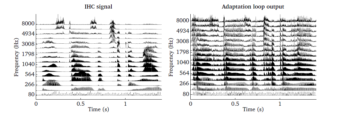
Fig. 25 Illustration of the adaptation processor. IHC output (left panel) as the
input to the adaptation processor and the corresponding output using
adpt_model=’adt_dau’ (right panel).
| [Dau1997a] | (1, 2) Dau, T., Püschel, D., and Kohlrausch, A. (1997a), “Modeling auditory processing of amplitude modulation. I. Detection and masking with narrow-band carriers,” Journal of the Acoustical Society of America 102(5), pp. 2892–2905. |
| [Pueschel1988] | (1, 2) Püschel, D. (1988), “Prinzipien der zeitlichen Analyse beim Hören,” Ph.D. thesis, University of Göttingen. |
| [Smith1977] | Smith, R. L. (1977), “Short-term adaptation in single auditory nerve fibers: some poststimulatory effects,” J Neurophysiol 40(5), pp. 1098–1111. |
| [Smith1983] | Smith, R. L., Brachman, M. L., and Goodman, D. a. (1983), “Adaptation in the Auditory Periphery,” Annals of the New York Academy of Sciences 405(1 Cochlear Pros), pp. 79–93. |