Amplitude modulation spectrogram (modulationProc.m)
The detection of envelope fluctuations is a very fundamental ability of the
human auditory system which plays a major role in speech perception.
Consequently, computational models have tried to exploit speech- and noise
specific characteristics of amplitude modulations by extracting so-called
amplitude modulation spectrogram (AMS)features with linearly-scaled modulation
filters [Kollmeier1994], [Tchorz2003], [Kim2009], [May2013a], [May2014a],
[May2014b]. The use of linearly-scaled modulation filters is, however, not
consistent with psychoacoustic data on modulation detection and masking in
humans [Bacon1989], [Houtgast1989], [Dau1997a], [Dau1997b], [Ewert2000]. As
demonstrated by [Ewert2000], the processing of envelope fluctuations can be
described effectively by a second-order band-pass filter bank with
logarithmically-spaced centre frequencies. Moreover, it has been shown that an
AMS feature representation based on an auditory-inspired modulation filter
bank with logarithmically-scaled modulation filters substantially improved the
performance of computational speech segregation in the presence of stationary
and fluctuating interferers [May2014c]. In addition, such a processing based on
auditory-inspired modulation filters has recently also been successful in speech
intelligibility prediction studies [Joergensen2011], [Joergensen2013]. To
investigate the contribution of both AMS feature representations, the
amplitude modulation processor can be used to extract linearly- and
logarithmically-scaled AMS features. Therefore, each frequency channel of the
IHC representation is analysed by a bank of modulation filters. The type of
modulation filters can be controlled by setting the parameter ams_fbType to
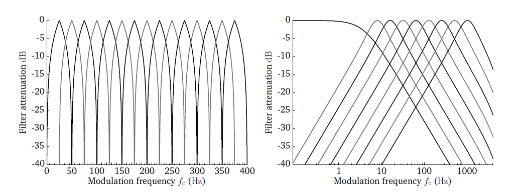
either ’lin’ or ’log’. To illustrate the difference between linear
linearly-scaled and logarithmically-scaled modulation filters, the corresponding
filter bank responses are shown in Fig. 34. The linear modulation
filter bank is implemented in the frequency domain, whereas the
logarithmically-scaled filter bank is realised by a band of second-order IIR
Butterworth filters with a constant-Q factor of 1. The modulation filter with
the lowest centre frequency is always implemented as a low-pass filter, as
illustrated in the right panel of Fig. 34.
Similarly to the gammatone processor described in Gammatone (gammatoneProc.m), there
are different ways to control the centre frequencies of the individual
modulation filters, which depend on the type of modulation filters
ams_fbType = 'lin'
- Specify
ams_lowFreqHz, ams_highFreqHz and ams_nFilter. The
requested number of filters ams_nFilter will be linearly-spaced
between ams_lowFreqHz and ams_highFreqHz. If ams_nFilter is
omitted, the number of filters will be set to 15 by default.
ams_fbType = 'log'
- Directly define a vector of centre frequencies, e.g.
ams_cfHz = [4 8 16
...]
. In this case, the parameters ams_lowFreqHz,
ams_highFreqHz, and ams_nFilter are ignored.
- Specify
ams_lowFreqHz and ams_highFreqHz. Starting at
ams_lowFreqHz, the centre frequencies will be logarithmically-spaced
at integer powers of two, e.g. 2^2, 2^3, 2^4 … until the
higher frequency limit ams_highFreqHz is reached.
- Specify
ams_lowFreqHz, ams_highFreqHz and ams_nFilter. The
requested number of filters ams_nFilter will be spaced logarithmically
as power of two between ams_lowFreqHz and ams_highFreqHz.
The temporal resolution at which the AMS features are computed is specified by
the window size ams_wSizeSec and the step size ams_hSizeSec. The window
size is an important parameter, because it determines how many periods of the
lowest modulation frequencies can be resolved within one individual time frame.
Moreover, the window shape can be adjusted by ams_wname. Finally, the IHC
representation can be downsampled prior to modulation analysis by selecting a
downsampling ratio ams_dsRatio larger than 1. A full list of AMS feature
parameters is shown in Table 31.
Table 31 List of parameters related to 'ams_features'.
| Parameter |
Default |
Description |
|---|
ams_fbType |
'log' |
Filter bank type ('lin' or 'log') |
ams_nFilter |
[] |
Number of modulation filters (integer) |
ams_lowFreqHz |
4 |
Lowest modulation filter centre frequency in Hz |
ams_highFreqHz |
1024 |
Highest modulation filter centre frequency in Hz |
ams_cfHz |
[] |
Vector of modulation filter centre frequencies in Hz |
ams_dsRatio |
4 |
Downsampling ratio of the IHC representation |
ams_wSizeSec |
32E-3 |
Window duration in s |
ams_hSizeSec |
16E-3 |
Window step size in s |
ams_wname |
'rectwin' |
Window name |
The functionality of the AMS feature processor is demonstrated by the script
DEMO_AMS and the corresponding four plots are presented in
Fig. 35. The time domain speech signal (top left panel) is
transformed into a IHC representation (top right panel) using 23 frequency
channels spaced between 80 and 8000 Hz. The linear and the logarithmic AMS
feature representations are shown in the bottom panels. The response of the
modulation filters are stacked on top of each other for each IHC frequency
channel, such that the AMS feature representations can be read like
spectrograms. It can be seen that the linear AMS feature representation is
more noisy in comparison to the logarithmically-scaled AMS features. Moreover,
the logarithmically-scaled modulation pattern shows a much higher correlation
with the activity reflected in the IHC representation.
| [Bacon1989] | Bacon, S. P. and Grantham, D. W. (1989), “Modulation masking: Effects of
modulation frequency, depths, and phase,” Journal of the Acoustical Society
of America 85(6), pp. 2575–2580. |
| [Dau1997b] | Dau, T., Püschel, D., and Kohlrausch, A. (1997b), “Modeling auditory
processing of amplitude modulation. II. Spectral and temporal integration,”
Journal of the Acoustical Society of America 102(5), pp. 2906–2919. |
| [Ewert2000] | (1, 2) Ewert, S. D. and Dau, T. (2000), “Characterizing frequency selectivity for
envelope fluctuations,” Journal of the Acoustical Society of America 108(3),
pp. 1181–1196. |
| [Houtgast1989] | Houtgast, T. (1989), “Frequency selectivity in amplitude-modulation
detection,” Journal of the Acoustical Society of America 85(4), pp.
1676–1680. |
| [Joergensen2013] | Jørgensen, S., Ewert, S. D., and Dau, T. (2013), “A multi-resolution
envelope-power based model for speech intelligibility,” Journal of the
Acoustical Society of America 134(1), pp. 1–11. |
| [Kim2009] | Kim, G., Lu, Y., Hu, Y., and Loizou, P. C. (2009), “An algorithm that
improves speech intelligibility in noise for normal-hearing listeners,”
Journal of the Acoustical Society of America 126(3), pp. 1486–1494. |
| [Kollmeier1994] | Kollmeier, B. and Koch, R. (1994), “Speech enhancement based on
physiological and psychoacoustical models of modulation perception and
binaural interaction,” Journal of the Acoustical Society of America 95(3),
pp. 1593–1602. |
| [May2013a] | May, T. and Dau, T. (2013), “Environment-aware ideal binary mask estimation
using monaural cues,” in IEEE Workshop on Applications of Signal Processing
to Audio and Acoustics (WASPAA), pp. 1–4. |
| [May2014a] | May, T. and Dau, T. (2014), “Requirements for the evaluation of
computational speech segregation systems,” Journal of the Acoustical Society
of America 136(6), pp. EL398– EL404. |
| [May2014b] | May, T. and Gerkmann, T. (2014), “Generalization of supervised learning for
binary mask estimation,” in International Workshop on Acoustic Signal
Enhancement, Antibes, France. |
| [May2014c] | May, T. and Dau, T. (2014), “Computational speech segregation based on an
auditory-inspired modulation analysis,” Journal of the Acoustical Society of
America 136(6), pp. 3350-3359. |