Computation of an auditory representation
The following sections describe how the Auditory front-end can be used to compute an auditory representation with default parameters of a given input signal. We will start with a simple example, and gradually explain how the user can gain more control over the respective parameters. It is assumed that the entire input signal - for which the auditory representation should be computed - is available. Therefore, this operation is referred to as batch processing. As stated before, the framework is also compatible with chunk-based processing (i.e., when the input signal is acquired continuously over time, but the auditory representation is computed for smaller signal chunks). The chunk-based processing will be explained in a later section.
Using default parameters
As an example, extracting the interaural level difference ’ild’ for a stereo
signal sIn (e.g., obtained from a ’.wav’ file through Matlab´s
wavread) sampled at a frequency fsHz (in Hz) can be done in the
following steps:
1 2 3 4 5 6 7 8 9 | % Instantiation of data and manager objects
dataObj = dataObject(sIn,fsHz);
managerObj = manager(dataObj);
% Request the computation of ILDs
sOut = managerObj.addProcessor('ild');
% Request the processing
managerObj.processSignal;
|
Line 2 and 3 show the instantiation of the two fundamental objects: the
data object and the manager. Note that the data object is always
instantiated first, as the manager needs a data object instance as input
argument to be constructed. The manager instance in line 3 is however an
“empty” instance of the manager class, in the sense that it will not
perform any processing. Hence a processing needs to be requested, as
done in line 6. This particular example will request the computation of
the inter-aural level difference ’ild’. This step is configuring the
manager instance managerObj to perform that type of processing, but
the processing itself is performed at line 9 by calling the
processSignal method of the manager class.
The request of an auditory representation via the addProcessor method of the
manager class on line 6 returns as an output argument a cell array containing a
handle to the requested signal, here named sOut. In the Auditory front-end, signals are
also objects. For example, for the output signal just generated:
>> sOut{1}

ans =

  TimeFrequencySignal with properties:

          cfHz: [1x31 double]
         Label: 'Interaural level difference'
          Name: 'ild'
    Dimensions: 'nSamples x nFilters'
          FsHz: 100
       Channel: 'mono'
          Data: [267x31 circVBufArrayInterface]
This shows the various properties of the signal object sOut. These
properties will be described in detail in the Technical description.
To access the
computed representation, e.g., for further processing, one can create a
copy of the data contained in the signal into a variable, say
myILDs:
>> myILDs = sOut{1}.Data(:);
Note
Note the use of the column operator (:). That is because the property
.Data of signal objects is not a conventional Matlab array and one needs
this syntax to access all the values it stores.
The nature of the .Data property is further described in
Circular buffer.
Input/output signals dimensions
The input signal sIn, for which a given auditory representation
needs be computed, is a simple array. Its first dimension (lines) should
span time. Its first column should correspond to the left channel (or
mono channel, if it is not a stereo signal) and the second column to the
right channel. This is typically the format returned by Matlab´s
embedded functions audioread and wavread.
The input signal can be either mono or stereo/binaural. The framework can operate on both. However, some representations, such as the as the ILD as requested in the previous example, are based on a comparison between the left and the right ear signals. If a mono signal was provided instead of a binaural signal, the request of computing the ILD representation would produce the following warning and the request would not be computed:
Warning: Cannot instantiate a binaural processor with a mono input signal!
> In manager>manager.addProcessor at 1127
The dimensions of the output signal from the addProcessor method
will depend on the representation requested. In the previous example,
the ’ild’ request returns a single output for a stereo input.
However, when the request is based on a single channel and the input is
stereo, the processing will be performed for left and right channel, and
both left and right outputs are returned. In such cases, the output from
the method addProcessor will be a cell array of dimensions 1 x 2
containing output signals for the left channel (first column) and right
channel (second column). For example, the returned sOut could take
the form:
>> sOut

sOut =

    [1x1 TimeFrequencySignal]    [1x1 TimeFrequencySignal]
The left-channel output can be accessed using sOut{1}, and
similarly, sOut{2} for the right-channel output.
Change parameters used for computation
For the requested representation
Each individual processors that is supported by the Auditory front-end can be controlled
by a set of parameters. Each parameter can be accessed by a unique
nametag and has a default value. A summary of all parameter names and
default values for the individual processors can be listed by the
command parameterHelper:
>> parameterHelper

Parameter handling in the TWO!EARS Auditory Front-End
-------------------------------------------------
The extraction of various auditory representations performed by the TWO!EARS Auditory Front-End software involves many parameters. Each parameter is given a unique name and a default value. When placing a request for TWO!EARS auditory front-end processing that uses one or more non-default parameters, a specific structure of non-default parameters needs to be provided as input. Such structure can be generated from |genParStruct|, using pairs of parameter name and chosen value as inputs.

Parameters names for each processor are listed below:
            Amplitude modulation|
            Auto-correlation|
            Cross-correlation|
            DRNL filterbank|
            Gabor features extractor|
            Gammatone filterbank|
            IC Extractor|
            ILD Extractor|
            ITD Extractor|
            Medial Olivo-Cochlear feedback processor|
            Inner hair-cell envelope extraction|
            Neural adaptation model|
            Offset detection|
            Offset mapping|
            Onset detection|
            Onset mapping|
            Pitch|
            Pre-processing stage|
            Precedence effect|
            Ratemap|
            Spectral features|
            Plotting parameters|
Each element in the list is a hyperlink, which will reveal the list of parameters for a given element, e.g.,
Inter-aural Level Difference Extractor parameters::

  Name            Default   Description
  ----            -------   -----------
  ild_wname       'hann'    Window name
  ild_wSizeSec    0.02      Window duration (s)
  ild_hSizeSec    0.01      Window step size (s)
It can be seen that the ILD processor can be controlled by three parameters,
namely ild_wname, ild_wSizeSec and ild_hSizeSec. A particular
parameter can be changed by creating a parameter structure which contains the
parameter name (nametags) and the corresponding value. The function
genParStruct can be used to create such a parameter structure. For
instance:
>> parameters = genParStruct('ild_wSizeSec',0.04,'ild_hSizeSec',0.02)

parameters =

  Parameters with properties:

    ild_hSizeSec: 0.0200
    ild_wSizeSec: 0.0400
will generate a suitable parameter structure parameters to request the
computation of ILD with a window duration of 40 ms and a step size of 20 ms.
This parameter structure is then passed as a second input argument in the
addProcessor method of a manager object. The previous example can be
rewritten considering the change in parameter values as follows:
% Instantiation of data and manager objects
dataObj = dataObject(sIn,fsHz);
managerObj = manager(dataObj);

% Non-default parameter values
parameters = genParStruct('ild_wSizeSec',0.04,'ild_hSizeSec',0.02);

% Place a request for the computation of ILDs
sOut = managerObj.addProcessor('ild',parameters);

% Perform processing
managerObj.processSignal;
For a dependency of the request
The previous example showed that the processor extracting ILDs was accepting three parameters. However, the representation it returns, the ILDs, will depend on more than these three parameters. For instance, it includes a certain number of frequency channels, but there is no parameter to control these in the ILD processor. That is because such parameters are from other processors that were used in intermediate steps to obtain the ILD. Controlling these parameters therefore requires knowledge of the individual steps in the processing.
Most auditory representations will depend on another representation,
itself being derived from yet another one. Thus, there is a chain of
dependencies between different representations, and multiple
processing stages will be required to compute a particular output. The
list of dependencies for a given processor can be visualised using the
function Processor.getDependencyList(’processorName’), e.g.
>> Processor.getDependencyList('ildProc')

ans =

    'innerhaircell'    'filterbank'    'time'
shows that the ILD depends on the inner hair-cell representation
(’innerhaircell’), which itself is obtained from the output of a gammatone
filter bank (’filterbank’). The filter bank is derived from the time-domain
signal, which itself has no further dependency as it is directly derived from
the input signal.
When placing a request to the manager, the user can also request a change in
parameters of any of the request’s dependencies. For example, the number of
frequency channels in the ILD representation is a property of the filter bank,
controlled by the parameter ’fb_nChannels’. (which name can be found using
parameterHelper.m). This parameter can also be requested to have a
non-default value, although it is not a parameter of the processor in charge of
computing the ILD. This is done in the same way as previously shown:
% Non-default parameter values
parameters = genParStruct('fb_nChannels',16);

% Place a request for the computation of ILDs
sOut = managerObj.addProcessor('ild',parameters);

% Perform processing
managerObj.processSignal;
The resulting ILD representation stored in sOut{1} will be based on 16
channels, instead of 31.
Compute multiple auditory representations
Place multiple requests
Multiple requests are supported in the framework, and can be carried
out by consecutive calls to the addProcessor method of an instance
of the manager with a single request argument. It is also possible to
have a single call to the addProcessor method with a cell array of
requests, e.g.:
% Place a request for the computation of ILDs AND autocorrelation
[sOut1 sOut2] = managerObj.addProcessor({'ild','autocorrelation'})
This way, the manager set up in the previous example will extract an ILD and
an auto-correlation representation, and provide handles to the three signals, in
sOut1{1} for the ILD (it is a mono representation), sOut2{1} and
sOut2{2} for the autocorrelations of respectively left and right channels.
To use non-default parameter values, three syntax are possible:
If there are several requests, but all use the same set of parameter values
p:managerObj.addProcessor({'name1', .. ,'nameN'},p)
If there is only one request (
name), but with different sets of parameter values (p1,…,pN), e.g., for investigating the influence of a given parametermanagerObj.addProcessor('name',{p1, .. ,pN})
If there are several requests and some, or all, of them use a different set of parameter values, then it is necessary to have a set of parameter (
p1,…,pN) for each request (possibly by duplicating the common ones) and place them in a cell array as follows:managerObj.addProcessor({'name1', .. ,'nameN'},{p1, .. ,pN})
Note that in the two examples above, no output is specified for the
addProcessor method, but the representations will be computed
nonetheless. The output of addProcessor is there for convenience and
the following subsection will explain how to get a hang on the computed
signals without an explicit output from addProcessor.
Requests can also be placed directly as optional arguments in the manager constructor, e.g., to reproduce the previous script example:
% Instantiation of data and manager objects
dataObj = dataObject(sIn,fsHz);
managerObj = manager(dataObj,{'ild','autocorrelation'});
The three possibilities described above can also be used in this syntax form.
Computing the signals
This is done in the exact same way as for a single request, by calling
the processSignal method of the manager:
% Perform processing
managerObj.processSignal;
Access internal signals
The optional output of the addProcessor method is provided for
convenience. It is actually a pointer (or handle, in Matlab´s terms) to
the actual signal object which is hosted by the data object on which the
manager is based. Once the processing is carried out, the properties of
the data object can be inspected:
>> dataObj

dataObj =

  dataObject with properties:

   bufferSize_s: 10
       isStereo: 1
            ild: {[1x1 TimeFrequencySignal]}
  innerhaircell: {[1x1 TimeFrequencySignal]  [1x1 TimeFrequencySignal]}
          input: {[1x1 TimeDomainSignal]  [1x1 TimeDomainSignal]}
           time: {[1x1 TimeDomainSignal]  [1x1 TimeDomainSignal]}
     filterbank: {[1x1 TimeFrequencySignal]  [1x1 TimeFrequencySignal]}
autocorrelation: {[1x1 CorrelationSignal]  [1x1 CorrelationSignal]}
Apart from the properties bufferSize_s and isStereo which are inherent
properties of the data object (and discussed later in the
Technical description), the remaining properties each correspond
to one of the representations computed to achieve the user’s request(s). They
are each arranged in cell arrays, with first column being the left, or mono
channel, and the second column the right channel. For instance, to get a handle
sGammaR to the right channel of the gammatone filter bank output, type:
>> sGammaR = dataObj.filterbank{2}

sGammaR =

  TimeFrequencySignal with properties:

      cfHz: [1x31 double]
     Label: 'Gammatone filterbank output'
      Name: 'filterbank'
Dimensions: 'nSamples x nFilters'
      FsHz: 44100
   Channel: 'right'
      Data: [118299x31 circVBufArrayInterface]
How to plot the result
Plotting auditory representations is made very easy in the Auditory front-end. As explained
before, each representation that was computed during a session is stored as a
signal object, which each are individual properties of the data object. Signal
objects of each type have a plot method. Called without any input
arguments, signal.plot will adequately plot the representation stored in
signal in a new figure, and returns as output a handle to said figure. The
plotting method for all signals can accept at least one optional argument, which
is a handle to an already existing figure or subplot in a figure. This way the
representation can be included in an existing plot. A second optional argument
is a structure of non-default plot parameters. The parameterHelper script
also lists plotting options, and they can be modified in the same way as
processor parameters, via the script genParStruct. These concepts can be
summed up in the following example lines, that follows right after the demo code
from the previous subsection:
1 2 3 4 5 6 7 8 9 10 11 12 13 14 15 16 17 18 19 20 21 | % Request the processing
managerObj.processSignal;
% Plot the ILDs in a separate figure
sOut{1}.plot;
% Create an empty figure with subplots
figure;
h1 = subplot(2,2,1);
h2 = subplot(2,2,2);
h3 = subplot(2,2,3);
h4 = subplot(2,2,4);
% Change plotting options to remove colorbar and reduce title size
p = genParStruct('bColorbar',0,'fsize_title',12);
% Plot additional representations
dataObj.innerhaircell{1}.plot(h1,p);
dataObj.innerhaircell{2}.plot(h2,p);
dataObj.filterbank{1}.plot(h3,p);
dataObj.filterbank{2}.plot(h4,p);
|
This script will produce the two figure windows displayed in Fig. 14. Line 22 of the script creates the window “Figure 1”, while lines 35 to 38 populate the window “Figure 2” which was created earlier (in lines 25 to 29).
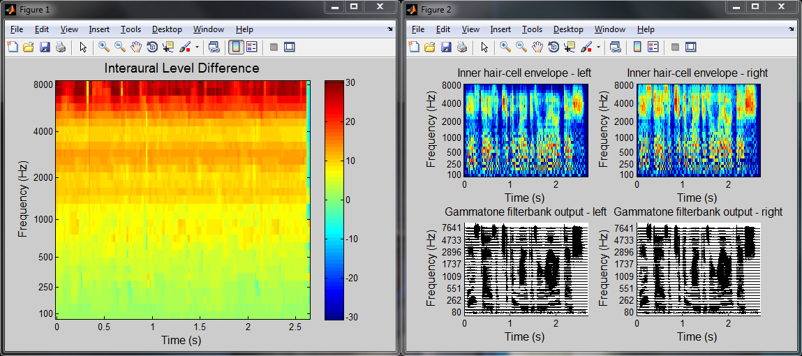
Fig. 14 The two example figures generated by the demo script.