Pre-processing (preProc.m)
Prior to computing any of the supported auditory representations, the input signal stored in the data object can be pre-processed with one of the following elements:
The order of processing is fixed. However, individual stages can be activated or deactivated, depending on the requirement of the user. The output is a time domain signal representation that is used as input to the next processors. Moreover, a list of adjustable parameters is listed in Table 18.
| Parameter | Default | Description |
|---|---|---|
pp_bRemoveDC |
false |
Activate DC removal filter |
pp_cutoffHzDC |
20 |
Cut-off frequency in Hz of the high-pass filter |
pp_bPreEmphasis |
false |
Activate pre-emphasis filter |
pp_coefPreEmphasis |
0.97 |
Coefficient of first-order high-pass filter |
pp_bNormalizeRMS |
false |
Activate RMS normalisation |
pp_intTimeSecRMS |
2 |
Time constant in s used for RMS estimation |
pp_bBinauralRMS |
true |
Link RMS normalisation across both ear signals |
pp_bLevelScaling |
false |
Apply level scaling to the given reference |
pp_refSPLdB |
100 |
Reference dB SPL to correspond to the input RMS |
pp_bMiddleEarFiltering |
false |
Apply middle ear filtering |
pp_middleEarModel |
'jepsen' |
Middle ear filter model |
The influence of each individual pre-processing stage except for the level
scaling is illustrated in Fig. 18, which can be reproduced by
running the script DEMO_PreProcessing.m. Panel 1 shows the left and the
right ears signals of two sentences at two different levels. The ear signals are
then mixed with a sinusoid at 0.5 Hz to simulate an interfering humming noise.
This humming can be effectively removed by the DC removal filter, as shown in
panel 3. Panel 4 shows the influence of the pre-emphasis stage. The AGC can be
used to equalise the long-term RMS level difference between the two sentences.
However, if the level difference between both ear signals should be preserved,
it is important to synchronise the AGC across both channels, as illustrated in
panel 5 and 6. Panel 7 shows the influence of the level scaling when using a
reference value of 100 dB SPL. Panel 8 shows the signals after middle ear
filtering, as the stapes motion velocity. Each individual pre-processing stage
is described in the following subsections.
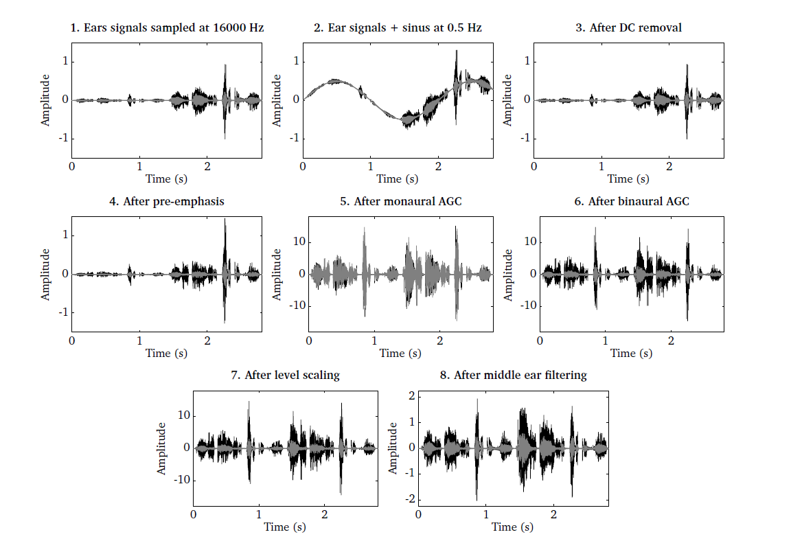
Fig. 18 Illustration of the individual pre-processing steps. 1) Ear signals consisting of two sentences recorded at different levels, 2) ear signals mixed with a 0.5 Hz humming, 3) ear signals after DC removal filter, 4) influence of pre-emphasis filter, 5) monaural RMS normalisation, 6) binaural RMS normalisation, 7) level scaling and 8) middle ear filtering.
DC removal filter
To remove low-frequency humming, a DC removal filter can be activated by using
the flag pp_bRemoveDC = true. The DC removal filter is based on a
fourth-order IIR Butterworth filter with a
cut-off frequency of 20 Hz, as specified by the parameter pp_cutoffHzDC =
20.
Pre-emphasis
A common pre-processing stage in the context of ASR includes a signal
whitening. The goal of this pre-processing stage is to roughly compensate for
the decreased energy at higher frequencies (e.g. due to lip radiation).
Therefore, a first-order FIR high-pass filter
is employed, where the filter coefficient pp_coefPreEmphasis determines the
amount of pre-emphasis and is typically selected from the range between 0.9 and
1. Here, we set the coefficient to pp_coefPreEmphasis = 0.97 by default
according to [Young2006]. This pre-emphasis filter can be activated by
setting the flag pp_bPreEmphasis = true.
RMS normalisation
A signal level normalisation stage is available which can be used to equalise
long-term level differences (e.g. when recording two speakers at two different
distances). For some applications, such as ASR and speaker identification
systems, it can be advantageous to maintain a constant signal power, such that
the features extracted by subsequent processors are invariant to the overall
signal level. To achieve this, the input signal is normalised by its RMS value
that has been estimated by a first-order low-pass filter with a time constant of
pp_intTimeSecRMS = 2. Such a normalisation stage has also been suggested in
the context of AMS feature
extraction [Tchorz2003], which are described in
Amplitude modulation spectrogram (modulationProc.m). The choice of the time constant is
a balance between maintaining the level fluctuations across individual words and
allowing the normalisation stage to follow sudden level changes.
The normalisation can be either applied independently for the left and the right
ear signal by setting the parameter pp_bBinauralRMS = false, or the
processing can be linked across ear signals by setting pp_bBinauralRMS =
true. When being used in the binaural mode, the larger RMS value of both ear
signals is used for normalisation, which will preserve the binaural cues (e.g.
ITD and ILD) that are encoded in the signal. The RMS normalisation can be
activated by the parameter pp_bNormalizeRMS = true.
Level reference and scaling
This stage is designed to implement the effect of calibration, in which the
amplitude of the incoming digital signal is matched to sound pressure in the
physical domain. This operation is necessary when any of the Auditory front-end models
requires the input to be represented in physical units (such as pascals, see the
middle ear filtering stage below). Within the current Auditory front-end framework, the
DRNL filter bank model requires this signal representation (see
Dual-resonance non-linear filter bank (drnlProc.m)). The request for this is given by setting
pp_bApplyLevelScaling = true, with a reference value pp_refSPLdB in dB
SPL which should correspond to the input RMS of 1. Then the input signal is
scaled accordingly, if it had been calibrated to a different reference. The
default value of pp_refSPLdB is 100, which corresponds to the convention
used in the work of [Jepsen2008]. The implementation is adopted from the
Auditory Modeling Toolbox [Soendergaard2013].
Middle ear filtering
This stage corresponds to the operation of the middle ear where the vibration
from the eardrum is transformed into the stapes motion. The filter model is
based on the findings from the measurement of human stapes displacement by
[Godde1994]. Its implementation is adopted from the Auditory Modeling Toolbox
[Soendergaard2013], which derives the stapes velocity as the output
[Lopez-Poveda2001], [Jepsen2008]. The input is assumed to be the eardrum
pressure represented in pascals which in turn assumes prior calibration. This
input-output representation in physical units is required particularly when the
DRNL filter bank model is used for the BM operation, because of its
level-dependent nonlinearity, designed based on that representation (see
Dual-resonance non-linear filter bank (drnlProc.m)). When including the middle-ear filtering in combination with
the linear gammatone filter, only the simple band-pass characteristic of this
model is needed without the need for input calibration or consideration of the
input/output units. The middle ear filtering can be applied by setting
pp_bMiddleEarFiltering = true. The filter data from [Lopez-Poveda2001] or
from [Jepsen2008] can be used for the processing, by specifying the model
pp_middleEarModel = 'lopezpoveda' or pp_middleEarModel = 'jepsen'
respectively.
| [Godde1994] | Goode, R. L., Killion, M., Nakamura, K., and Nishihara, S. (1994), “New knowledge about the function of the human middle ear: development of an improved analog model.” The American journal of otology 15(2), pp. 145–154. |
| [Tchorz2003] | Tchorz, J. and Kollmeier, B. (2003), “SNR estimation based on amplitude modulation analysis with applications to noise suppression,” IEEE Transactions on Audio, Speech, and Language Processing 11(3), pp. 184–192. |
| [Young2006] | Young, S., Evermann, G., Gales, M., Hain, T., Kershaw, D., Liu, X., Moore, G., Odell, J., Ollason, D., Povey, D., Valtchev, V., and Woodland, P. (2006), The HTK Book (for HTK Version 3.4), Cambridge University Engineering Department, http://htk.eng.cam.ac.uk. |