Auditory filter bank
One central processing element of the Auditory front-end is the separation of incoming
acoustic signals into different spectral bands, as it happens in the human inner
ear. In psychoacoustic modelling, two different approaches have been followed
over the years. One is the simulation of this stage by a linear filter bank
composed of gammatone filters. This linear gammatone filter bank can be
considered a standard element for auditory models and has therefore been
included in the framework. A computationally more challenging, but at the same
time physiologically more plausible simulation of this process can be realised
by a nonlinear BM model, and we have implemented the DRNL model, as
developed by [Meddis2001]. The filter bank representation is requested by
using the name tag 'filterbank'. The filter bank type can be controlled by
the parameter fb_type. To select a gammatone filter bank, fb_type should
be set to ’gammatone’ (which is the default), whereas the DRNL filter bank
is used when setting fb_type = 'drnl'. Some of the parameters are common to
the two filter bank, while some are specific, in which case their value is
disregarded if the other type of filter bank was requested.
Table 19 summarises all parameters corresponding to
the 'filterbank' request. Parameters specific to a filter bank type are
separated by a horizontal line. The two filter bank implementations are
described in detail in the following two subsections, along with their
corresponding parameters.
| Parameter | Default | Description |
|---|---|---|
fb_type |
'gammatone' |
Filter bank type, 'gammatone' or 'drnl' |
fb_lowFreqHz |
80 |
Lowest characteristic frequency in Hz |
fb_highFreqHz |
8000 |
Highest characteristic frequency in Hz |
fb_nERBs |
1 |
Distance between adjacent filters in ERB |
fb_nChannels |
[] |
Number of frequency channels |
fb_cfHz |
[] |
Vector of characteristic frequencies in Hz |
fb_nGamma |
4 |
Filter order, 'gammatone'-only |
fb_bwERBs |
1.01859 |
Filter bandwidth in ERB, 'gammatone'-only |
fb_lowFreqHz |
80 |
Lowest characteristic frequency in Hz, 'gammatone'-only |
fb_mocIpsi |
1 |
Ipsilateral MOC factor (0 to 1). Given as a scalar (across all frequency channels) or a vector (individual per frequency channel), |
fb_mocContra |
1 |
Contralateral MOC factor (0 to 1). Same format as
|
fb_model |
'CASP' |
DRNL model (reserved
for future extension), 'drnl'-only |
Gammatone (gammatoneProc.m)
The time domain signal can be processed by a bank of gammatone filters that
simulates the frequency selective properties of the human BM. The
corresponding Matlab function is adopted from the Auditory Modeling Toolbox
[Soendergaard2013]. The gammatone filters cover a frequency range between
fb_lowFreqHz and fb_highFreqHz and are linearly spaced on the ERB
scale [Glasberg1990]. In addition, the distance between adjacent filter centre
frequencies on the ERB scale can be specified by fb_nERBs, which
effectively controls the frequency resolution of the gammatone filter bank.
There are three different ways to control the centre frequencies of the
individual gammatone filters:
- Define a vector with centre frequencies, e.g.
fb_cfHz = [100 200 500
...]
. In this case, the parametersfb_lowFreqHz,fb_highFreqHz,fb_nERBsandfb_nChannelsare ignored. - Specify
fb_lowFreqHz,fb_highFreqHzandfb_nChannels. The requested number of filtersfb_nChannelswill be spaced betweenfb_lowFreqHzandfb_highFreqHz. The centre frequencies of the first and the last filter will match withfb_lowFreqHzandfb_highFreqHz, respectively. To accommodate an arbitrary number of filters, the spacing between adjacent filtersfb_nERBswill be automatically adjusted. Note that this changes the overlap between neighbouring filters. - It is also possible to specify
fb_lowFreqHz,fb_highFreqHzandfb_nERBs. Starting atfb_lowFreqHz, the centre frequencies will be spaced at a distance offb_nERBson the ERB scale until the specified frequency range is covered. The centre frequency of the last filter will not necessarily match withfb_highFreqHz.
The filter order, which determines the slope of the filter skirts, is set to
fb_nGamma = 4 by default. The bandwidths of the gammatone filters depend on
the filter order and the centre frequency, and the default scaling factor for a
forth-order filter is approximately fb_bwERBs = 1.01859. When adjusting the
parameter fb_bwERBs, it should be noted that the resulting filter shape will
deviate from the original gammatone filter as measured by [Glasberg1990]. For
instance, increasing fb_bwERBs leads to a broader filter shape. A full list
of parameters is shown in Table 19.
The gammatone filter bank is illustrated in Fig. 19, which has
been produced by the script DEMO_Gammatone.m. The speech signal shown in
the left panel is passed through a bank of 16 gammatone filters spaced between
80 Hz and 8000 Hz. The output of each individual filter is shown in the right
panel.
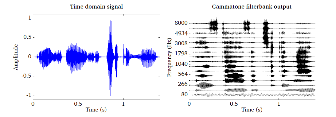
Fig. 19 Time domain signal (left panel) and the corresponding output of the gammatone processor consisting of 16 auditory filters spaced between 80 Hz and 8000 Hz (right panel).
Given the output of the gammatone filterbank, it is possible to reconstruct the
original input signal by compensating for the frequency-specific delay of the
individual subband signals. First, the peak in the envelope domain can be aligned
across all subband channels by introducing a frequency-specific time lead
[BrownCooke94]. In addition, a phase compensation factor is necessary to align
the peak in the fine structure across channels [BrownCooke94]. The gammatone
processor in the Auditory front-end supports this phase compensation strategy, which can be
activated by the flag fb_bAlign.
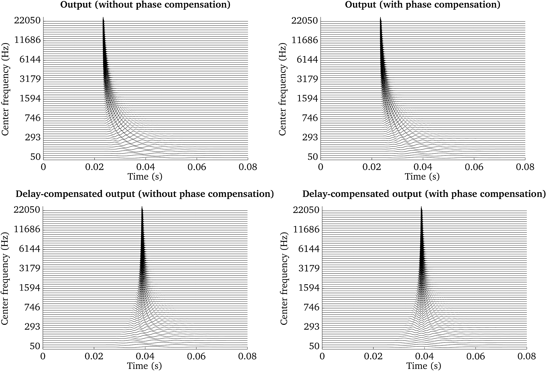
Fig. 20 Frequency-specific output of a gammatone filterbank: without phase and delay compensation (top left panel), with phase compensation (top right panel), with delay compensation (bottom left panel) and with delay and phase compensation (bottom right panel).
The impact of these different strategies is visualized in
Fig. 20 and Fig. 21, which have been
produced by the script Demo_Gammatone_Reconstruction.m. The four panels in
Fig. 20 show the frequency-specific output of a gammatone
filterbank consisting of 64 filters spaced between 50 and 22050 Hz in response
to an impulse located at 23.2 ms. The top left panel shows the output without
delay and phase compensation. The impact of the phase compensation can be seen
in the top right panel, which ensures that the fine structure of the subband
signals is aligned across channels. The additional effect of the delay
compensation can be seen in the bottom left and bottom right panels without and
with phase compensation.
Finally, the compensation of the time delay can be combined with a frequency-specific gain factor to ensure a flat frequency response of the analysis-synthesis system [Hohmann2002]. The impulse response and frequency response of three gammatone-based analysis-synthesis systems is presented in Fig. 21. The output refers to a delay-compensated gammatone filterbank without phase compensation, which produces the largest deviations when comparing it to the response of the input signal. The addition of the phase compensation allows for a reasonably flat frequency response, although the absolute magnitude is shifted with respect to the original input. When combining all three stages, namely the delay, phase and gain compensation, a flat frequency response close to 0 dB can be achieved.
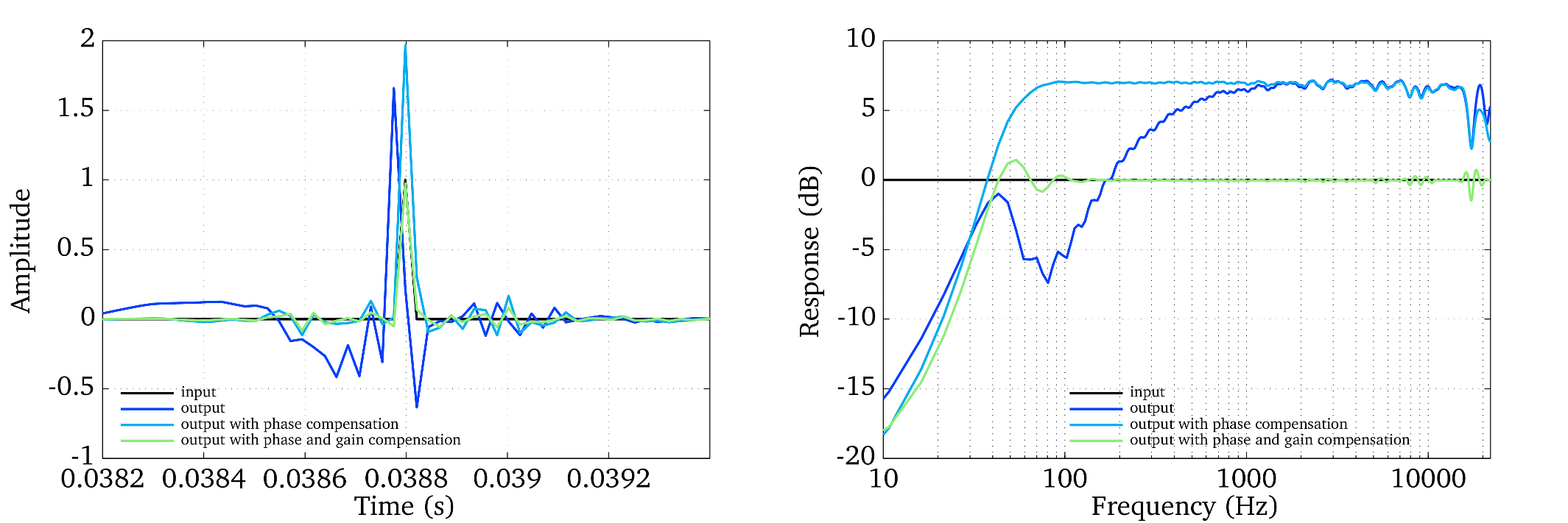
Fig. 21 Impulse response (left panel) and frequency response (right panel) of an impulse (input signal) and three gammatone-based analysis-synthesis systems.
Dual-resonance non-linear filter bank (drnlProc.m)
The DRNL filter bank models the nonlinear operation of the cochlear, in
addition to the frequency selective feature of the BM. The DRNL processor
was motivated by attempts to better represent the nonlinear operation of the
BM in the modelling, and allows for testing the performance of peripheral
models with the BM nonlinearity and MOC feedback in comparison to that with
the conventional linear BM model. All the internal representations that depend
on the BM output can be extracted using the DRNL processor in the dependency
chain in place of the gammatone filter bank. This can reveal the implication of
the BM nonlinearity and MOC feedback for activities such as speech
perception in noise (see [Brown2010] for example) or source localisation. It is
expected that the use of a nonlinear model, together with the adaptation loops
(see Adaptation (adaptationProc.m)), will reduce the influence of overall level on the
internal representations and extracted features. In this sense, the use of the
DRNL model is a physiologically motivated alternative for a linear BM model
where the influence of level is typically removed by the use of a level
normalisation stage (see AGC in Pre-processing (preProc.m) for example). The
structure of DRNL filter bank is based on the work of [Meddis2001]. The
frequencies corresponding to the places along the BM, over which the responses
are to be derived and observed, are specified as a list of characteristic
frequencies fb_cfHz. For each characteristic frequency channel, the time
domain input signal is passed through linear and nonlinear paths, as seen in
Fig. 22. Currently the implementation follows the model
defined as CASP by [Jepsen2008], in terms of the detailed structure and
operation, which is specified by the default argument 'CASP' for
fb_model.
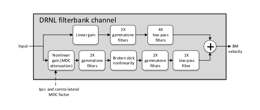
Fig. 22 Filter bank channel structure, following the model specification as default, with an additional nonlinear gain stage to receive feedback.
In the CASP model, the linear path consists of a gain stage, two cascaded gammatone filters, and four cascaded low-pass filters; the nonlinear path consists of a gain (attenuation) stage, two cascaded gammatone filters, a ’broken stick’ nonlinearity stage, two more cascaded gammatone filters, and a low-pass filter. The outputs at the two paths are then summed as the BM output motion. These sub-modules and their individual parameters (e.g., gammatone filter centre frequencies) are specific to the model and hidden to the users. Details regarding the original idea behind the parameter derivation can be found in [Lopez-Poveda2001], which the CASP model slightly modified to provide a better fit of the output to physiological findings from human cochlear research works.
The MOC feedback is implemented in an open-loop structure within the DRNL
filter bank model as the gain factor to be applied to the nonlinear path. This
approach is used by [Ferry2007], where the attenuation caused by MOC the
feedback at each of the filter bank channels is controlled externally by the
user. Two additional input arguments are introduced for this feature:
fb_mocIpsi and fb_mocContra. These represent the amount of reflexive
feedback through the ipsilateral and contralateral paths, in the form of a
factor from 0 to 1 that the nonlinear path input signal is multiplied by in
conjunction. Conceptually, fb_mocIpsi = 1 and fb_mocContra = 1 would
mean that no attenuation is applied to the nonlinear path input, and
fb_mocIpsi = 0 and fb_mocContra = 0 would mean that the nonlinear path
is totally eliminated. Table 19 summarises the
parameters for DRNL the processor that can be controlled by the user. Note
that fb_cfHz corresponds to the characteristic frequencies and not the
centre frequencies as used in the gammatone filter bank, although they can
have the same values for comparison. Otherwise, the characteristic frequencies
can be generated in the same way as the centre frequencies for the gammatone
filter bank.
Fig. 23 shows the BM stage output at 1 kHz characteristic
frequency using the DRNL processor (on the right hand side), compared to that
using the gammatone filter bank (left hand side), based on the right ear input
signal shown in panel 1 of Fig. 18 (speech excerpt repeated twice
with a level difference). The plots can be generated by running the script
DEMO_DRNL.m. It should be noted that the CASP model of DRNL filter bank
expects the input signal to be transformed to the middle ear stapes velocity
before processing. Therefore, for direct comparison of the outputs in this
example, the same pre-processing was applied for the gammatone filter bank
(stapes velocity was used as the input, through the level scaling and middle ear
filtering). It is seen that the level difference between the initial speech
component and its repetition is reduced with the nonlinearity incorporated,
compared to the gammatone filter bank output, which shows the compressive nature
of the nonlinear model responding to input level changes as described earlier.
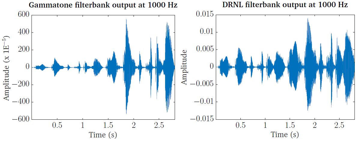
Fig. 23 The gammatone processor output (left panel) compared to the output of the DRNL processor (right panel), based on the right ear signal shown in panel 1 of Fig. 18, at 1 kHz centre or characteristic frequency. Note that the input signal is converted to the stapes velocity before entering both processors for direct comparison. The level difference between the two speech excerpts is reduced in the DRNL response, showing its compressive nature to input level variations.
| [BrownCooke94] | (1, 2) Brown, G. J. and Cooke, M. P. (1994), “Computational auditory scene analysis .” Computer Speech and Language 8(4), pp. 297–336. |
| [Brown2010] | Brown, G. J., Ferry, R. T., and Meddis, R. (2010), “A computer model of auditory efferent suppression: implications for the recognition of speech in noise.” The Journal of the Acoustical Society of America 127(2), pp. 943–954. |
| [Ferry2007] | Ferry, R. T. and Meddis, R. (2007), “A computer model of medial efferent suppression in the mammalian auditory system,” The Journal of the Acoustical Society of America 122(6), pp. 3519-3526. |
| [Glasberg1990] | (1, 2) Glasberg, B. R. and Moore, B. C. J. (1990), “Derivation of auditory filter shapes from notched-noise data,” Hearing Research 47(1-2), pp. 103–138. |
| [Hohmann2002] |
|
| [Jepsen2008] | Jepsen, M. L., Ewert, S. D., and Dau, T. (2008), “A computational model of human auditory signal processing and perception.” Journal of the Acoustical Society of America 124(1), pp. 422–438. |
| [Lopez-Poveda2001] | Lopez-Poveda, E. A. and Meddis, R. (2001), “A human nonlinear cochlear filterbank,” Journal of the Acoustical Society of America 110(6), pp. 3107–3118. |
| [Soendergaard2013] | Søndergaard, P. L. and Majdak, P. (2013), “The auditory modeling toolbox,” in The Technology of Binaural Listening, edited by J. Blauert, Springer, Heidelberg–New York NY–Dordrecht–London, chap. 2, pp. 33–56. |