Available processors
This section presents a detailed description of all processors that are
currently supported by the Auditory front-end framework. Each processor can be controlled by
a set of parameters, which will be explained and all default settings will be
listed. Finally, a demonstration will be given, showing the functionality of
each processor. The corresponding Matlab files are contained in the Auditory front-end folder
/test and can be used to reproduce the individual plots. A full list of
available processors can be displayed by using the command requestList. An
overview of the commands for instantiating processors is given in
Computation of an auditory representation.
- Pre-processing (
preProc.m) - Auditory filter bank
- Inner hair-cell (
ihcProc.m) - Adaptation (
adaptationProc.m) - Auto-correlation (
autocorrelationProc.m) - Rate-map (
ratemapProc.m) - Spectral features (
spectralFeaturesProc.m) - Onset strength (
onsetProc.m) - Offset strength (
offsetProc.m) - Binary onset and offset maps (
transientMapProc.m) - Pitch (
pitchProc.m) - Amplitude modulation spectrogram (
modulationProc.m) - Spectro-temporal modulation spectrogram
- Cross-correlation (
crosscorrelationProc.m) - Interaural time differences (
itdProc.m) - Interaural level differences (
ildProc.m) - Interaural coherence (
icProc.m)
Pre-processing (preProc.m)
Prior to computing any of the supported auditory representations, the input signal stored in the data object can be pre-processed with one of the following elements:
- DC bias removal
- Pre-emphasis
- RMS normalisation using an automatic gain control
- Level scaling to a pre-defined SPL reference
- Middle ear filtering
The order of processing is fixed. However, individual stages can be activated or deactivated, depending on the requirement of the user. The output is a time domain signal representation that is used as input to the next processors. Moreover, a list of adjustable parameters is listed in Table 4.
| Parameter | Default | Description |
|---|---|---|
pp_bRemoveDC |
false |
Activate DC removal filter |
pp_cutoffHzDC |
20 |
Cut-off frequency in Hz of the high-pass filter |
pp_bPreEmphasis |
false |
Activate pre-emphasis filter |
pp_coefPreEmphasis |
0.97 |
Coefficient of first-order high-pass filter |
pp_bNormalizeRMS |
false |
Activate RMS normalisation |
pp_intTimeSecRMS |
2 |
Time constant in s used for RMS estimation |
pp_bBinauralRMS |
true |
Link RMS normalisation across both ear signals |
pp_bLevelScaling |
false |
Apply level scaling to the given reference |
pp_refSPLdB |
100 |
Reference dB SPL to correspond to the input RMS |
pp_bMiddleEarFiltering |
false |
Apply middle ear filtering |
pp_middleEarModel |
'jepsen' |
Middle ear filter model |
The influence of each individual pre-processing stage except for the level
scaling is illustrated in Fig. 7, which can be reproduced by
running the script DEMO_PreProcessing.m. Panel 1 shows the left and the
right ears signals of two sentences at two different levels. The ear signals are
then mixed with a sinusoid at 0.5 Hz to simulate an interfering humming noise.
This humming can be effectively removed by the DC removal filter, as shown in
panel 3. Panel 4 shows the influence of the pre-emphasis stage. The AGC can be
used to equalise the long-term RMS level difference between the two sentences.
However, if the level difference between both ear signals should be preserved,
it is important to synchronise the AGC across both channels, as illustrated in
panel 5 and 6. Panel 7 shows the influence of the level scaling when using a
reference value of 100 dB SPL. Panel 8 shows the signals after middle ear
filtering, as the stapes motion velocity. Each individual pre-processing stage
is described in the following subsections.
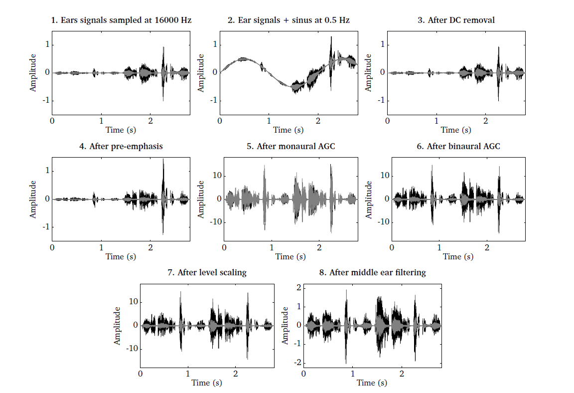
Fig. 7 Illustration of the individual pre-processing steps. 1) Ear signals consisting of two sentences recorded at different levels, 2) ear signals mixed with a 0.5 Hz humming, 3) ear signals after DC removal filter, 4) influence of pre-emphasis filter, 5) monaural RMS normalisation, 6) binaural RMS normalisation, 7) level scaling and 8) middle ear filtering.
DC removal filter
To remove low-frequency humming, a DC removal filter can be activated by using
the flag pp_bRemoveDC = true. The DC removal filter is based on a
fourth-order IIR Butterworth filter with a
cut-off frequency of 20 Hz, as specified by the parameter pp_cutoffHzDC =
20.
Pre-emphasis
A common pre-processing stage in the context of ASR includes a signal
whitening. The goal of this pre-processing stage is to roughly compensate for
the decreased energy at higher frequencies (e.g. due to lip radiation).
Therefore, a first-order FIR high-pass filter
is employed, where the filter coefficient pp_coefPreEmphasis determines the
amount of pre-emphasis and is typically selected from the range between 0.9 and
1. Here, we set the coefficient to pp_coefPreEmphasis = 0.97 by default
according to [Young2006]. This pre-emphasis filter can be activated by
setting the flag pp_bPreEmphasis = true.
RMS normalisation
A signal level normalisation stage is available which can be used to equalise
long-term level differences (e.g. when recording two speakers at two different
distances). For some applications, such as ASR and speaker identification
systems, it can be advantageous to maintain a constant signal power, such that
the features extracted by subsequent processors are invariant to the overall
signal level. To achieve this, the input signal is normalised by its RMS value
that has been estimated by a first-order low-pass filter with a time constant of
pp_intTimeSecRMS = 2. Such a normalisation stage has also been suggested in
the context of AMS feature
extraction [Tchorz2003], which are described in
Amplitude modulation spectrogram (modulationProc.m). The choice of the time constant is
a balance between maintaining the level fluctuations across individual words and
allowing the normalisation stage to follow sudden level changes.
The normalisation can be either applied independently for the left and the right
ear signal by setting the parameter pp_bBinauralRMS = false, or the
processing can be linked across ear signals by setting pp_bBinauralRMS =
true. When being used in the binaural mode, the larger RMS value of both ear
signals is used for normalisation, which will preserve the binaural cues (e.g.
ITD and ILD) that are encoded in the signal. The RMS normalisation can be
activated by the parameter pp_bNormalizeRMS = true.
Level reference and scaling
This stage is designed to implement the effect of calibration, in which the
amplitude of the incoming digital signal is matched to sound pressure in the
physical domain. This operation is necessary when any of the Auditory front-end models
requires the input to be represented in physical units (such as pascals, see the
middle ear filtering stage below). Within the current Auditory front-end framework, the
DRNL filter bank model requires this signal representation (see
Dual-resonance non-linear filter bank (drnlProc.m)). The request for this is given by setting
pp_bApplyLevelScaling = true, with a reference value pp_refSPLdB in dB
SPL which should correspond to the input RMS of 1. Then the input signal is
scaled accordingly, if it had been calibrated to a different reference. The
default value of pp_refSPLdB is 100, which corresponds to the convention
used in the work of [Jepsen2008]. The implementation is adopted from the
Auditory Modeling Toolbox [Soendergaard2013].
Middle ear filtering
This stage corresponds to the operation of the middle ear where the vibration
from the eardrum is transformed into the stapes motion. The filter model is
based on the findings from the measurement of human stapes displacement by
[Godde1994]. Its implementation is adopted from the Auditory Modeling Toolbox
[Soendergaard2013], which derives the stapes velocity as the output
[Lopez-Poveda2001], [Jepsen2008]. The input is assumed to be the eardrum
pressure represented in pascals which in turn assumes prior calibration. This
input-output representation in physical units is required particularly when the
DRNL filter bank model is used for the BM operation, because of its
level-dependent nonlinearity, designed based on that representation (see
Dual-resonance non-linear filter bank (drnlProc.m)). When including the middle-ear filtering in combination with
the linear gammatone filter, only the simple band-pass characteristic of this
model is needed without the need for input calibration or consideration of the
input/output units. The middle ear filtering can be applied by setting
pp_bMiddleEarFiltering = true. The filter data from [Lopez-Poveda2001] or
from [Jepsen2008] can be used for the processing, by specifying the model
pp_middleEarModel = 'lopezpoveda' or pp_middleEarModel = 'jepsen'
respectively.
Auditory filter bank
One central processing element of the Auditory front-end is the separation of incoming
acoustic signals into different spectral bands, as it happens in the human inner
ear. In psychoacoustic modelling, two different approaches have been followed
over the years. One is the simulation of this stage by a linear filter bank
composed of gammatone filters. This linear gammatone filter bank can be
considered a standard element for auditory models and has therefore been
included in the framework. A computationally more challenging, but at the same
time physiologically more plausible simulation of this process can be realised
by a nonlinear BM model, and we have implemented the DRNL model, as
developed by [Meddis2001]. The filter bank representation is requested by
using the name tag 'filterbank'. The filter bank type can be controlled by
the parameter fb_type. To select a gammatone filter bank, fb_type should
be set to ’gammatone’ (which is the default), whereas the DRNL filter bank
is used when setting fb_type = 'drnl'. Some of the parameters are common to
the two filter bank, while some are specific, in which case their value is
disregarded if the other type of filter bank was requested.
Table 5 summarises all parameters corresponding to
the 'filterbank' request. Parameters specific to a filter bank type are
separated by a horizontal line. The two filter bank implementations are
described in detail in the following two subsections, along with their
corresponding parameters.
| Parameter | Default | Description |
|---|---|---|
fb_type |
'gammatone' |
Filter bank type, 'gammatone' or 'drnl' |
fb_lowFreqHz |
80 |
Lowest characteristic frequency in Hz |
fb_highFreqHz |
8000 |
Highest characteristic frequency in Hz |
fb_nERBs |
1 |
Distance between adjacent filters in ERB |
fb_nChannels |
[] |
Number of frequency channels |
fb_cfHz |
[] |
Vector of characteristic frequencies in Hz |
fb_nGamma |
4 |
Filter order, 'gammatone'-only |
fb_bwERBs |
1.01859 |
Filter bandwidth in ERB, 'gammatone'-only |
fb_lowFreqHz |
80 |
Lowest characteristic frequency in Hz, 'gammatone'-only |
fb_mocIpsi |
1 |
Ipsilateral MOC factor (0 to 1). Given as a scalar (across all frequency channels) or a vector (individual per frequency channel), |
fb_mocContra |
1 |
Contralateral MOC factor (0 to 1). Same format as
|
fb_model |
'CASP' |
DRNL model (reserved
for future extension), 'drnl'-only |
Gammatone (gammatoneProc.m)
The time domain signal can be processed by a bank of gammatone filters that
simulates the frequency selective properties of the human BM. The
corresponding Matlab function is adopted from the Auditory Modeling Toolbox
[Soendergaard2013]. The gammatone filters cover a frequency range between
fb_lowFreqHz and fb_highFreqHz and are linearly spaced on the ERB
scale [Glasberg1990]. In addition, the distance between adjacent filter centre
frequencies on the ERB scale can be specified by fb_nERBs, which
effectively controls the frequency resolution of the gammatone filter bank.
There are three different ways to control the centre frequencies of the
individual gammatone filters:
- Define a vector with centre frequencies, e.g.
fb_cfHz = [100 200 500
...]
. In this case, the parametersfb_lowFreqHz,fb_highFreqHz,fb_nERBsandfb_nChannelsare ignored. - Specify
fb_lowFreqHz,fb_highFreqHzandfb_nChannels. The requested number of filtersfb_nChannelswill be spaced betweenfb_lowFreqHzandfb_highFreqHz. The centre frequencies of the first and the last filter will match withfb_lowFreqHzandfb_highFreqHz, respectively. To accommodate an arbitrary number of filters, the spacing between adjacent filtersfb_nERBswill be automatically adjusted. Note that this changes the overlap between neighbouring filters. - It is also possible to specify
fb_lowFreqHz,fb_highFreqHzandfb_nERBs. Starting atfb_lowFreqHz, the centre frequencies will be spaced at a distance offb_nERBson the ERB scale until the specified frequency range is covered. The centre frequency of the last filter will not necessarily match withfb_highFreqHz.
The filter order, which determines the slope of the filter skirts, is set to
fb_nGamma = 4 by default. The bandwidths of the gammatone filters depend on
the filter order and the centre frequency, and the default scaling factor for a
forth-order filter is approximately fb_bwERBs = 1.01859. When adjusting the
parameter fb_bwERBs, it should be noted that the resulting filter shape will
deviate from the original gammatone filter as measured by [Glasberg1990]. For
instance, increasing fb_bwERBs leads to a broader filter shape. A full list
of parameters is shown in Table 5.
The gammatone filter bank is illustrated in Fig. 8, which has
been produced by the script DEMO_Gammatone.m. The speech signal shown in
the left panel is passed through a bank of 16 gammatone filters spaced between
80 Hz and 8000 Hz. The output of each individual filter is shown in the right
panel.
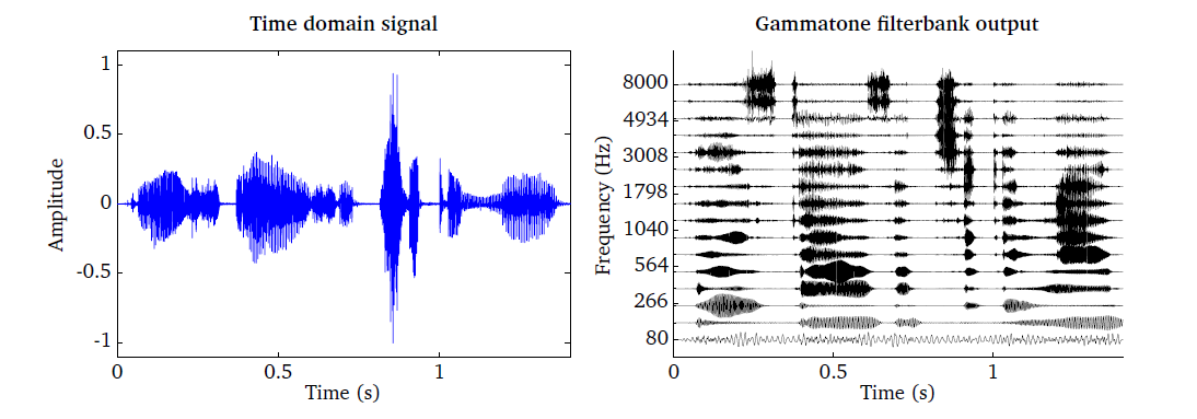
Fig. 8 Time domain signal (left panel) and the corresponding output of the gammatone processor consisting of 16 auditory filters spaced between 80 Hz and 8000 Hz (right panel).
Dual-resonance non-linear filter bank (drnlProc.m)
The DRNL filter bank models the nonlinear operation of the cochlear, in
addition to the frequency selective feature of the BM. The DRNL processor
was motivated by attempts to better represent the nonlinear operation of the
BM in the modelling, and allows for testing the performance of peripheral
models with the BM nonlinearity and MOC feedback in comparison to that with
the conventional linear BM model. All the internal representations that depend
on the BM output can be extracted using the DRNL processor in the dependency
chain in place of the gammatone filter bank. This can reveal the implication of
the BM nonlinearity and MOC feedback for activities such as speech
perception in noise (see [Brown2010] for example) or source localisation. It is
expected that the use of a nonlinear model, together with the adaptation loops
(see Adaptation (adaptationProc.m)), will reduce the influence of overall level on the
internal representations and extracted features. In this sense, the use of the
DRNL model is a physiologically motivated alternative for a linear BM model
where the influence of level is typically removed by the use of a level
normalisation stage (see AGC in Pre-processing (preProc.m) for example). The
structure of DRNL filter bank is based on the work of [Meddis2001]. The
frequencies corresponding to the places along the BM, over which the responses
are to be derived and observed, are specified as a list of characteristic
frequencies fb_cfHz. For each characteristic frequency channel, the time
domain input signal is passed through linear and nonlinear paths, as seen in
Fig. 9. Currently the implementation follows the model
defined as CASP by [Jepsen2008], in terms of the detailed structure and
operation, which is specified by the default argument 'CASP' for
fb_model.
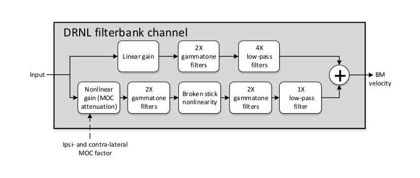
Fig. 9 Filter bank channel structure, following the model specification as default, with an additional nonlinear gain stage to receive feedback.
In the CASP model, the linear path consists of a gain stage, two cascaded gammatone filters, and four cascaded low-pass filters; the nonlinear path consists of a gain (attenuation) stage, two cascaded gammatone filters, a ’broken stick’ nonlinearity stage, two more cascaded gammatone filters, and a low-pass filter. The outputs at the two paths are then summed as the BM output motion. These sub-modules and their individual parameters (e.g., gammatone filter centre frequencies) are specific to the model and hidden to the users. Details regarding the original idea behind the parameter derivation can be found in [Lopez-Poveda2001], which the CASP model slightly modified to provide a better fit of the output to physiological findings from human cochlear research works.
The MOC feedback is implemented in an open-loop structure within the DRNL
filter bank model as the gain factor to be applied to the nonlinear path. This
approach is used by [Ferry2007], where the attenuation caused by MOC the
feedback at each of the filter bank channels is controlled externally by the
user. Two additional input arguments are introduced for this feature:
fb_mocIpsi and fb_mocContra. These represent the amount of reflexive
feedback through the ipsilateral and contralateral paths, in the form of a
factor from 0 to 1 that the nonlinear path input signal is multiplied by in
conjunction. Conceptually, fb_mocIpsi = 1 and fb_mocContra = 1 would
mean that no attenuation is applied to the nonlinear path input, and
fb_mocIpsi = 0 and fb_mocContra = 0 would mean that the nonlinear path
is totally eliminated. Table 5 summarises the
parameters for DRNL the processor that can be controlled by the user. Note
that fb_cfHz corresponds to the characteristic frequencies and not the
centre frequencies as used in the gammatone filter bank, although they can
have the same values for comparison. Otherwise, the characteristic frequencies
can be generated in the same way as the centre frequencies for the gammatone
filter bank.
Fig. 10 shows the BM stage output at 1 kHz characteristic
frequency using the DRNL processor (on the right hand side), compared to that
using the gammatone filter bank (left hand side), based on the right ear input
signal shown in panel 1 of Fig. 7 (speech excerpt repeated twice
with a level difference). The plots can be generated by running the script
DEMO_DRNL.m. It should be noted that the CASP model of DRNL filter bank
expects the input signal to be transformed to the middle ear stapes velocity
before processing. Therefore, for direct comparison of the outputs in this
example, the same pre-processing was applied for the gammatone filter bank
(stapes velocity was used as the input, through the level scaling and middle ear
filtering). It is seen that the level difference between the initial speech
component and its repetition is reduced with the nonlinearity incorporated,
compared to the gammatone filter bank output, which shows the compressive nature
of the nonlinear model responding to input level changes as described earlier.
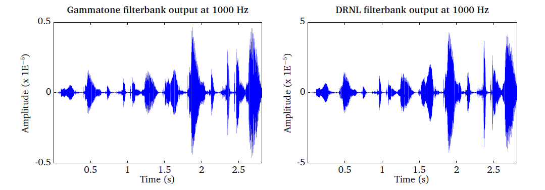
Fig. 10 The gammatone processor output (left panel) compared to the output of the DRNL processor (right panel), based on the right ear signal shown in panel 1 of Fig. 7, at 1 kHz centre or characteristic frequency. Note that the input signal is converted to the stapes velocity before entering both processors for direct comparison. The level difference between the two speech excerpts is reduced in the DRNL response, showing its compressive nature to input level variations.
Inner hair-cell (ihcProc.m)
The IHC functionality is simulated by extracting the envelope of the output of
individual gammatone filters. The corresponding IHC function is adopted from
the Auditory Modeling Toolbox [Soendergaard2013]. Typically, the envelope is extracted by
combining half-wave rectification and low-pass filtering. The low-pass filter is
motivated by the loss of phase-locking in the auditory nerve at higher
frequencies [Bernstein1996], [Bernstein1999]. Depending on the cut-off
frequency of the IHC models, it is possible to control the amount of
fine-structure information that is present in higher frequency channels. The
cut-off frequency and the order of the corresponding low-pass filter vary across
methods and a complete overview of supported IHC models is given in
Table 6. A particular model can be selected by using the
parameter ihc_method.
ihc_method |
Description |
|---|---|
'hilbert' |
Hilbert transform |
'halfwave' |
Half-wave rectification |
'fullwave' |
Full-wave rectification |
'square' |
Squared |
'dau' |
Half-wave rectification and low-pass filtering at 1000 Hz [Dau1996] |
'joergensen' |
Hilbert transform and low-pass filtering at 150 Hz [Joergensen2011] |
'breebart' |
Half-wave rectification and low-pass filtering at 770 Hz [Breebart2001] |
'bernstein' |
Half-wave rectification, compression and low-pass filtering at 425 Hz [Bernstein1999] |
The effect of the IHC processor is demonstrated in Fig. 11, where
the output of the gammatone filter bank is compared with the output of an IHC
model by running the script DEMO_IHC.m. Whereas individual peaks are
resolved in the lowest channel of the IHC output, only the envelope is
retained at higher frequencies.
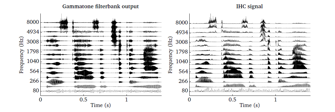
Fig. 11 Illustration of the envelope extraction processor. BM output (left panel)
and the corresponding IHC model output using ihc_method = ’dau’ (right
panel).
Adaptation (adaptationProc.m)
This processor corresponds to the adaptive response of the auditory nerve fibers, in which abrupt changes in the input result in emphasised overshoots followed by gradual decay to compressed steady-state level [Smith1977], [Smith1983]. The function is adopted from the Auditory Modeling Toolbox [Soendergaard2013]. The adaptation stage is modelled as a chain of five feedback loops in series. Each of the loops consists of a low-pass filter with its own time constant, and a division operator [Pueschel1988], [Dau1996], [Dau1997a]. At each stage, the input is divided by its low-pass filtered version. The time constant affects the charging / releasing state of the filter output at a given moment, and thus affects the amount of attenuation caused by the division. This implementation realises the characteristics of the process that input variations which are rapid compared to the time constants are linearly transformed, whereas stationary input signals go through logarithmic compression.
| Parameter | Default | Description |
|---|---|---|
adpt_lim |
10 |
Overshoot limiting ratio |
adpt_mindB |
0 |
Lowest audible threshold of the signal in dB SPL |
adpt_tau |
[0.005
0.050
0.129
0.253
0.500] |
Time constants of feedback loops |
adpt_model |
'adt_dau' |
Implementation model
can be used instead of the above three parameters (See Table 8) |
The adaptation processor uses three parameters to generate the output from the
IHC representation: adpt_lim determines the maximum ratio of the onset
response amplitude against the steady-state response, which sets a limit to the
overshoot caused by the loops. adpt_mindB sets the lowest audible threshold
of the input signal. adpt_tau are the time constants of the loops. Though
the default model uses five loops and thus five time constants, variable number
of elements of adpt_tau is supported which can vary the number of loops.
Some specific sets of these parameters, as used in related studies, are also
supported optionally with the adpt_model parameter. This can be given
instead of the other three parameters, which will set them as used by the
respective researchers. Table 7 lists the
parameters and their default values, and Table 8 lists
the supported models. The output signal is expressed in MU which deviates the
input-output relation from a perfect logarithmic transform, such that the input
level increment at low level range results in a smaller output level increment
than the input increment at higher level range. This corresponds to a smaller
just-noticeable level change at high levels than at low levels [Dau1996],
[Jepsen2008], with the use of DRNL model for the BM stage, introduces an
additional squaring expansion process between the IHC output and the
adaptation stage, which transforms the input that comes through the DRNL-IHC
processors into an intensity-like representation to be compatible with the
adaptation implementation originally designed based on the use of gammatone
filter bank. The adaptation processor recognises whether DRNL or gammatone
processor is used in the chain and adjusts the input signal accordingly.
adpt_model |
Description |
|---|---|
'adt_dau' |
Choose the parameters as in the models of [Dau1996], [Dau1997a]. This consists of 5 adaptation loops with an overshoot limit of 10 and a minimum level of 0 dB. This is a correction in regard to the model described in [Dau1996], which did not use overshoot limiting. The adaptation loops have an exponentially spaced time constants
|
'adt_puschel' |
Choose the parameters as in the original model [Pueschel1988]. This consists of 5 adaptation loops without overshoot limiting ( constants |
'adt_breebaart' |
As 'adt_puschel', but with overshoot limiting |
The effect of the adaptation processor - the exaggeration of rapid variations -
is demonstrated in Fig. 12, where the output of the IHC model
from the same input as used in the example of Inner hair-cell (ihcProc.m) (the right
panel of Fig. 11) is compared to the adaptation output by running the
script DEMO_Adaptation.m.
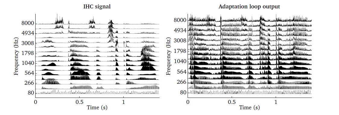
Fig. 12 Illustration of the adaptation processor. IHC output (left panel) as the
input to the adaptation processor and the corresponding output using
adpt_model=’adt_dau’ (right panel).
Auto-correlation (autocorrelationProc.m)
Auto-correlation is an important computational concept that has been extensively
studied in the context of predicting human pitch perception [Licklider1951],
[Meddis1991]. To measure the amount of periodicity that is present in
individual frequency channels, the ACF is computed in the FFT domain for
short time frames based on the IHC representation. The unbiased ACF
scaling is used to account for the fact that fewer terms contribute to the ACF
at longer time lags. The resulting ACF is normalised by the ACF at lag zero
to ensure values between minus one and one. The window size ac_wSizeSec
determines how well low-frequency pitch signals can be reliably estimated and
common choices are within the range of 10 milliseconds – 30 milliseconds.
For the purpose of pitch estimation, it has been suggested to modify the signal
prior to correlation analysis in order to reduce the influence of the formant
structure on the resulting ACF [Rabiner1977]. This pre-processing can be
activated by the flag ac_bCenterClip and the following nonlinear operations
can be selected for ac_ccMethod: centre clip and compress ’clc’, centre
clip ’cc’, and combined centre and peak clip ’sgn’. The percentage of
centre clipping is controlled by the flag ac_ccAlpha, which sets the
clipping level to a fixed percentage of the frame-based maximum signal level.
A generalised ACF has been suggested by [Tolonen2000], where the exponent
ac\_K can be used to control the amount of compression that is applied to
the ACF. The conventional ACF function is computed using a value of
ac\_K=2, whereas the function is compressed when a smaller value than 2 is
used. The choice of this parameter is a trade-off between sharpening the peaks
in the resulting ACF function and amplifying the noise floor. A value of
ac\_K = 2/3 has been suggested as a good compromise [Tolonen2000]. A list
of all ACF-related parameters is given in Table 9. Note
that these parameters will influence the pitch processor, which is described in
Pitch (pitchProc.m).
| Parameter | Default | Description |
|---|---|---|
ac_wname |
'hann' |
Window type |
ac_wSizeSec |
0.02 |
Window duration in s |
ac_hSizeSec |
0.01 |
Window step size in s |
ac_bCenterClip |
false |
Activate centre clipping |
ac_clipMethod |
'clp' |
Centre clipping method 'clc', 'clp', or 'sgn' |
ac_clipAlpha |
0.6 |
Centre clipping threshold within [0,1] |
ac_K |
2 |
Exponent in ACF |
A demonstration of the ACF processor is shown in Fig. 13, which has
been produced by the scrip DEMO_ACF.m. It shows the IHC output in
response to a 20 ms speech signal for 16 frequency channels (left panel). The
corresponding ACF is presented in the upper right panel, whereas the SACF is
shown in the bottom right panel. Prominent peaks in the SACF indicate lag
periods which correspond to integer multiples of the fundamental frequency of
the analysed speech signal. This relationship is exploited by the pitch
processor, which is described in Pitch (pitchProc.m).
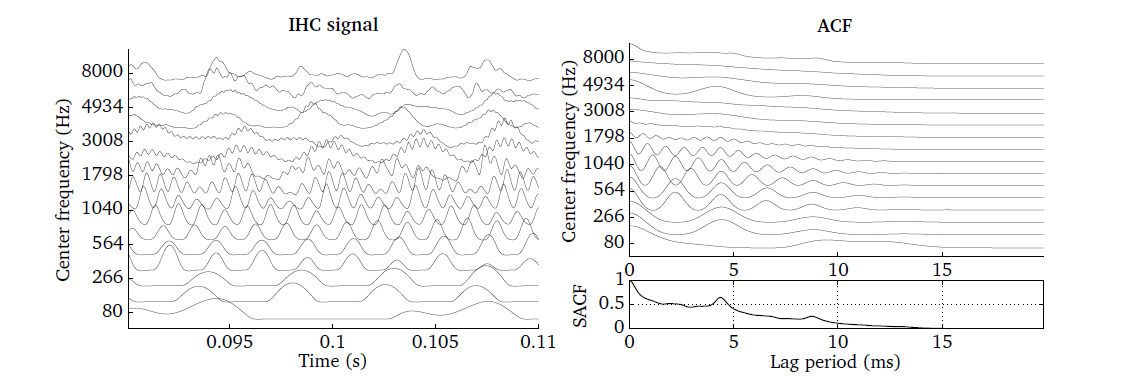
Fig. 13 IHC representation of a speech signal shown for one time frame of 20 ms duration (left panel) and the corresponding ACF (right panel). The SACF summarises the ACF across all frequency channels (bottom right panel).
Rate-map (ratemapProc.m)
The rate-map represents a map of auditory nerve firing rates [Brown1994] and is
frequently employed as a spectral feature in CASA systems [Wang2006], ASR
[Cooke2001] and speaker identification systems [May2012]. The rate-map is
computed for individual frequency channels by smoothing the IHC signal
representation with a leaky integrator that has a time constant of typically
rm\_decaySec=8 ms. Then, the smoothed IHC signal is averaged across all
samples within a time frame and thus the rate-map can be interpreted as an
auditory spectrogram. Depending on whether the rate-map scaling rm_scaling
has been set to ’magnitude’ or ’power’, either the magnitude or the
squared samples are averaged within each time frame. The temporal resolution can
be adjusted by the window size rm_wSizeSec and the step size
rm_hSizeSec. Moreover, it is possible to control the shape of the window
function rm_wname, which is used to weight the individual samples within a
frame prior to averaging. The default rate-map parameters are listed in
Table 10.
| Parameter | Default | Description |
|---|---|---|
'rm_wname' |
'hann' |
Window type |
'rm_wSizeSec' |
0.02 |
Window duration in s |
'rm_hSizeSec' |
0.01 |
Window step size in s |
'rm_scaling' |
'power' |
Rate-map scaling ('magnitude' or 'power') |
'rm_decaySec' |
0.008 |
Leaky integrator time constant in s |
The rate-map is demonstrated by the script DEMO_Ratemap and the
corresponding plots are presented in Fig. 14. The IHC
representation of a speech signal is shown in the left panel, using a bank of 64
gammatone filters spaced between 80 and 8000 Hz. The corresponding rate-map
representation scaled in dB is presented in the right panel.
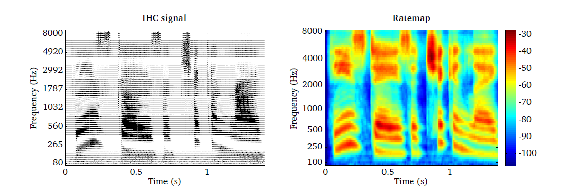
Fig. 14 IHC representation of s speech signal using 64 auditory filters (left panel) and the corresponding rate-map representation (right panel).
Spectral features (spectralFeaturesProc.m)
In order to characterise the spectral content of the ear signals, a set of spectral features is available that can serve as a physical correlate to perceptual attributes, such as timbre and coloration [Peeters2011]. All spectral features summarise the spectral content of the rate-map representation across auditory filters and are computed for individual time frames. The following 14 spectral features are available:
'centroid': The spectral centroid represents the centre of gravity of the rate-map and is one of the most frequently-used timbre parameters [Tzanetakis2002], [Jensen2004], [Peeters2011]. The centroid is normalised by the highest rate-map centre frequency to reduce the influence of the gammatone parameters.'spread': The spectral spread describes the average deviation of the rate-map around its centroid, which is commonly associated with the bandwidth of the signal. Noise-like signals have usually a large spectral spread, while individual tonal sounds with isolated peaks will result in a low spectral spread. Similar to the centroid, the spectral spread is normalised by the highest rate-map centre frequency, such that the feature value ranges between zero and one.'brightness': The brightness reflects the amount of high frequency information and is measured by relating the energy above a pre-defined cutoff frequency to the total energy. This cutoff frequency is set tosf_br_cf = 1500Hz by default [Jensen2004], [Peeters2011]. This feature might be used to quantify the sensation of sharpness.'high-frequency content': The high-frequency content is another metric that measures the energy associated with high frequencies. It is derived by weighting each channel in the rate-map by its squared centre frequency and integrating this representation across all frequency channels [Jensen2004]. To reduce the sensitivity of this feature to the overall signal level, the high-frequency content feature is normalised by the rate-map integrated across-frequency.'crest': The SCM is defined as the ratio between the maximum value and the arithmetic mean and can be used to characterise the peakiness of the rate-map. The feature value is low for signals with a flat spectrum and high for a rate-map with a distinct spectral peak [Peeters2011], [Lerch2012].'decrease': The spectral decrease describes the average spectral slope of the rate-map representation, putting a stronger emphasis on the low frequencies [Peeters2011].'entropy': The entropy can be used to capture the peakiness of the spectral representation [Misra2004]. The resulting feature is low for a rate-map with many distinct spectral peaks and high for a flat rate-map spectrum.'flatness': The SFM is defined as the ratio of the geometric mean to the arithmetic mean and can be used to distinguish between harmonic (SFM is close to zero) and a noisy signals (SFM is close to one) [Peeters2011].'irregularity': The spectral irregularity quantifies the variations of the logarithmically-scaled rate-map across frequencies [Jensen2004].'kurtosis': The excess kurtosis measures whether the spectrum can be characterised by a Gaussian distribution [Lerch2012]. This feature will be zero for a Gaussian distribution.'skewness': The spectral skewness measures the symmetry of the spectrum around its arithmetic mean [Lerch2012]. The feature will be zero for silent segments and high for voiced speech where substantial energy is present around the fundamental frequency.'roll-off': Determines the frequency in Hz below which a pre-defined percentagesf_ro_percof the total spectral energy is concentrated. Common values for this threshold are betweensf_ro_perc = 0.85[Tzanetakis2002] andsf_ro_perc = 0.95[Scheirer1997], [Peeters2011]. The roll-off feature is normalised by the highest rate-map centre frequency and ranges between zero and one. This feature can be useful to distinguish voiced from unvoiced signals.'flux': The spectral flux evaluates the temporal variation of the logarithmically-scaled rate-map across adjacent frames [Lerch2012]. It has been suggested to be useful for the distinction of music and speech signals, since music has a higher rate of change [Scheirer1997].'variation': The spectral variation is defined as one minus the normalised correlation between two adjacent time frames of the rate-map [Peeters2011].
A list of all parameters is presented in Table 11.
| Parameter | Default | Description |
|---|---|---|
sf_requests |
'all' |
List of requested spectral features (e.g.
to display the full list of supported spectral features. |
sf_br_cf |
1500 |
Cut-off frequency in Hz for brightness feature |
sf_ro_perc |
0.85 |
Threshold (re. 1) for spectral roll-off feature |
The extraction of spectral features is demonstrated by the script
Demo_SpectralFeatures.m, which produces the plots shown in
Fig. 15. The complete set of 14 spectral features is
computed for the speech signal shown in the top left panel. Whenever the unit of
the spectral feature was given in frequency, the feature is shown in black in
combination with the corresponding rate-map representation.
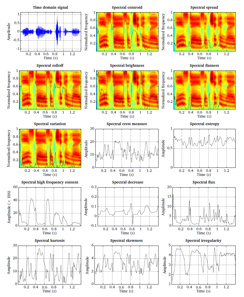
Fig. 15 Speech signal and 14 spectral features that were extracted based on the rate-map representation.
Onset strength (onsetProc.m)
According to [Bregman1990], common onsets and offsets across frequency are
important grouping cues that are utilised by the human auditory system to
organise and integrate sounds originating from the same source. The onset
processor is based on the rate-map representation, and therefore, the choice of
the rate-map parameters, as listed in Table 10, will influence the
output of the onset processor. The temporal resolution is controlled by the
window size rm_wSizeSec and the step size rm_hSizeSec, respectively. The
amount of temporal smoothing can be adjusted by the leaky integrator time
constant rm_decaySec, which reduces the amount of temporal fluctuations in
the rate-map. Onset are detected by measuring the frame-based increase in energy
of the rate-map representation. This detection is performed based on the
logarithmically-scaled energy, as suggested by [Klapuri1999]. It is possible to
limit the strength of individual onsets to an upper limit, which is by default
set to ons_maxOnsetdB = 30. A list of all parameters is presented in
Table 12.
| Parameter | Default | Description |
|---|---|---|
ons_maxOnsetdB |
30 |
Upper limit for onset strength in dB |
The resulting onset strength expressed in decibel, which is a function of time
frame and frequency channel, is shown in Fig. 16. The
two figures can be replicated by running the script DEMO_OnsetStrength.m.
When considering speech as an input signal, it can be seen that onsets appear
simultaneously across a broad frequency range and typically mark the beginning
of an auditory event.
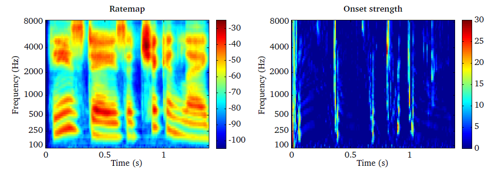
Fig. 16 Rate-map representation (left panel) of speech and the corresponding onset strength in decibel (right panel).
Offset strength (offsetProc.m)
Similarly to onsets, the strength of offsets can be estimated by measuring the
frame-based decrease in logarithmically-scaled energy. As discussed in the
previous section, the selected rate-map parameters as listed in
Table 10 will influence the offset processor. Similar to the onset
strength, the offset strength can be constrained to a maximum value of
ons_maxOffsetdB = 30. A list of all parameters is presented in
Table 12.
| Parameter | Default | Description |
|---|---|---|
ofs_maxOffsetdB |
30 |
Upper limit for offset strength in dB |
The offset strength is demonstrated by the script DEMO_OffsetStrength.m and
the corresponding figures are depicted in Fig. 17.
It can be seen that the overall magnitude of the offset strength is lower
compared to the onset strength. Moreover, the detected offsets are less
synchronised across frequency.
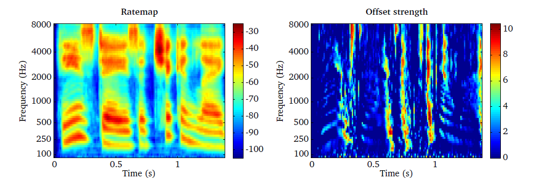
Fig. 17 Rate-map representation (left panel) of speech and the corresponding offset strength in decibel (right panel).
Binary onset and offset maps (transientMapProc.m)
The information about sudden intensity changes, as represented by onsets or
offsets, can be combined in order to organise and group the acoustic input
according to individual auditory events. The required processing is similar for
both onsets and offsets, and is summarised by the term transient detection. To
apply this transient detection based on the onset strength or offset strength,
the user should use the request name ’onset_map’ or ’offset_map’,
respectively. Based on the transient strength which is derived from the
corresponding onset strength and offset strength processor (described in
Onset strength (onsetProc.m) and Offset strength (offsetProc.m), a binary decision about transient
activity is formed, where only the most salient information is retained. To
achieve this, temporal and across-frequency constraints are imposed for the
transient information. Motivated by the observation that two sounds are
perceived as separated auditory events when the difference in terms of their
onset time is in the range of 20 ms – 40 ms [Turgeon2002], transients are fused
if they appear within a pre-defined time context. If two transients appear
within this time context, only the stronger one will be considered. This time
context can be adjusted by trm_fuseWithinSec. Moreover, the minimum
across-frequency context can be controlled by the parameters trm_minSpread.
To allow for this selection, individual transients which are connected across
multiple TF units are extracted using Matlab’s image labelling tool
bwlabel . The binary transient map will only retain those transients which
consists of at least trm_minSpread connected TF units. The salience of the
cue can be specified by the detection thresholds trm_minStrengthdB. Whereas
this thresholds control the required relative change, a global threshold
excludes transient activity if the corresponding rate-map level is below a
pre-defined threshold, as determined by trm_minValuedB. A summary of all
parameters is given in Table 14.
| Parameter | Default | Description |
|---|---|---|
trm_fuseWithinSec |
30E-3 |
Time constant below which transients are fused |
trm_minSpread |
5 |
Minimum number of connected TF units |
trm_minStrengthdB |
3 |
Minimum onset strength in dB |
trm_minValuedB |
-80 |
Minimum rate-map level in dB |
To illustrate the benefit of selecting onset and offset information, a rate-map
representation is shown in Fig. 18 (left panel), where the
corresponding onsets and offsets detected by the transientMapProc, through
two individual requests ’onset_map’ and ’offset_map’, and without
applying any temporal or across-frequency constraints are overlaid (respectively
in black and white). It can be seen that the onset and offset information is
quite noisy. When only retaining the most salient onsets and offsets by applying
temporal and across-frequency constraints (right panel), the remaining onsets
and offsets can be used as temporal markers, which clearly mark the beginning
and the end of individual auditory events.
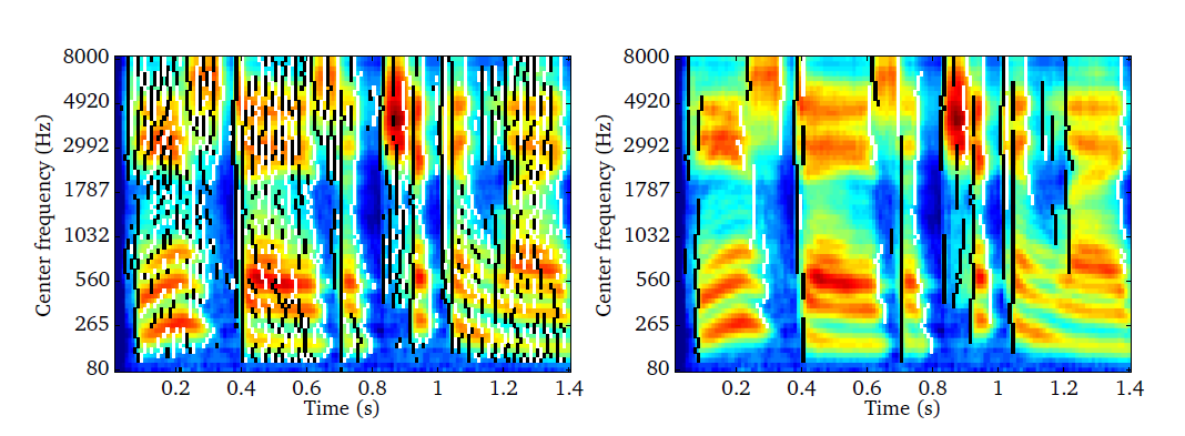
Fig. 18 Detected onsets and offsets indicated by the black and white vertical bars. The left panels shows all onset and offset events, whereas the right panel applies temporal and across-frequency constraints in order to retain the most salient onset and offset events.
Pitch (pitchProc.m)
Following [Slaney1990], [Meddis2001], [Meddis1997], the sub-band periodicity
analysis obtained by the ACF can be integrated across frequency by giving
equal weight to each frequency channel. The resulting SACF reflects the
strength of periodicity as a function of the lag period for a given time frame,
as illustrated in Fig. 13. Based on the SACF representation, the
most salient peak within the plausible pitch frequency range p_pitchRangeHz
is detected for each frame in order to obtain an estimation of the fundamental
frequency. In addition to the peak position, the corresponding amplitude of the
SACF is used to reflect the confidence of the underlying pitch estimation.
More specifically, if the SACF magnitude drops below a pre-defined percentage
p_confThresPerc of its global maximum, the corresponding pitch estimate is
considered unreliable and set to zero. The estimated pitch contour is smoothed
across time frames by a median filter of order p_orderMedFilt, which aims at
reducing the amount of octave errors. A list of all parameters is presented in
Table 15. In the context of pitch estimation, it will be useful to
experiment with the settings related to the non-linear pre-processing of the
ACF, as described in Auto-correlation (autocorrelationProc.m).
| Parameter | Default | Description |
|---|---|---|
p_pitchRangeHz |
[80 400] |
Plausible pitch frequency range in Hz |
p_confThresPerc |
0.7 |
Confidence threshold related to the SACF magnitude |
p_orderMedFilt |
3 |
Order of the median filter |
The task of pitch estimation is demonstrated by the script DEMO_Pitch and
the corresponding SACF plots are presented in Fig. 19. The pitch
is estimated for an anechoic speech signal (top left panel). The corresponding
is presented in the top right panel, where each black cross represents the most
salient lag period per time frame. The plausible pitch range is indicated by the
two white dashed lines. The confidence measure of each individual pitch
estimates is shown in the bottom left panel, which is used to set the estimated
pitch to zero if the magnitude of the SACF is below the threshold. The final
pitch contour is post-processed with a median filter and shown in the bottom
right panel. Unvoiced frames, where no pitch frequency was detected, are
indicated by NaN‘s.
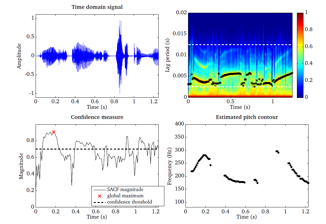
Fig. 19 Time domain signal (top left panel) and the corresponding SACF (top right panel). The confidence measure based on the SACF magnitude is used to select reliable pitch estimates (bottom left panel). The final pitch estimate is post-processed by a median filter (bottom right panel).
Amplitude modulation spectrogram (modulationProc.m)
The detection of envelope fluctuations is a very fundamental ability of the
human auditory system which plays a major role in speech perception.
Consequently, computational models have tried to exploit speech- and noise
specific characteristics of amplitude modulations by extracting so-called
amplitude modulation spectrogram (AMS)features with linearly-scaled modulation
filters [Kollmeier1994], [Tchorz2003], [Kim2009], [May2013a], [May2014a],
[May2014b]. The use of linearly-scaled modulation filters is, however, not
consistent with psychoacoustic data on modulation detection and masking in
humans [Bacon1989], [Houtgast1989], [Dau1997a], [Dau1997b], [Ewert2000]. As
demonstrated by [Ewert2000], the processing of envelope fluctuations can be
described effectively by a second-order band-pass filter bank with
logarithmically-spaced centre frequencies. Moreover, it has been shown that an
AMS feature representation based on an auditory-inspired modulation filter
bank with logarithmically-scaled modulation filters substantially improved the
performance of computational speech segregation in the presence of stationary
and fluctuating interferers [May2014c]. In addition, such a processing based on
auditory-inspired modulation filters has recently also been successful in speech
intelligibility prediction studies [Joergensen2011], [Joergensen2013]. To
investigate the contribution of both AMS feature representations, the
amplitude modulation processor can be used to extract linearly- and
logarithmically-scaled AMS features. Therefore, each frequency channel of the
IHC representation is analysed by a bank of modulation filters. The type of
modulation filters can be controlled by setting the parameter ams_fbType to
either ’lin’ or ’log’. To illustrate the difference between linear
linearly-scaled and logarithmically-scaled modulation filters, the corresponding
filter bank responses are shown in Fig. 20. The linear modulation
filter bank is implemented in the frequency domain, whereas the
logarithmically-scaled filter bank is realised by a band of second-order IIR
Butterworth filters with a constant-Q factor of 1. The modulation filter with
the lowest centre frequency is always implemented as a low-pass filter, as
illustrated in the right panel of Fig. 20.
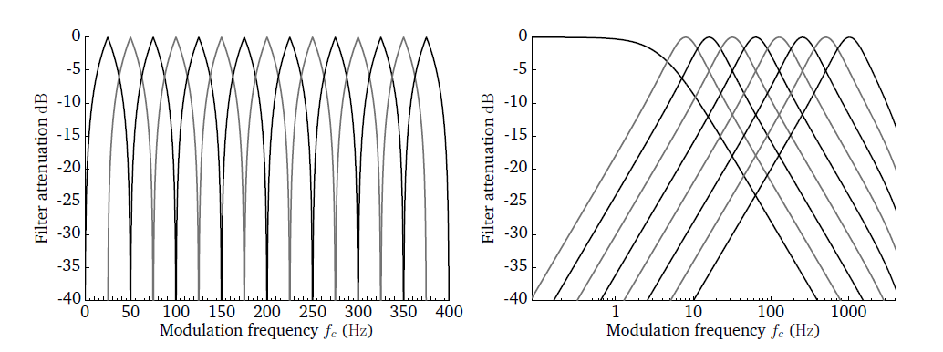
Fig. 20 Transfer functions of 15 linearly-scaled (left panel) and 9 logarithmically-scaled (right panel) modulation filters.
Similarly to the gammatone processor described in Gammatone (gammatoneProc.m), there are different ways to control the centre frequencies of the individual modulation filters, which depend on the type of modulation filters
ams_fbType = 'lin'- Specify
ams_lowFreqHz,ams_highFreqHzandams_nFilter. The requested number of filtersams_nFilterwill be linearly-spaced betweenams_lowFreqHzandams_highFreqHz. Ifams_nFilteris omitted, the number of filters will be set to 15 by default.
- Specify
ams_fbType = 'log'- Directly define a vector of centre frequencies, e.g.
ams_cfHz = [4 8 16
...]
. In this case, the parametersams_lowFreqHz,ams_highFreqHz, andams_nFilterare ignored. - Specify
ams_lowFreqHzandams_highFreqHz. Starting atams_lowFreqHz, the centre frequencies will be logarithmically-spaced at integer powers of two, e.g. 2^2, 2^3, 2^4 ... until the higher frequency limitams_highFreqHzis reached. - Specify
ams_lowFreqHz,ams_highFreqHzandams_nFilter. The requested number of filtersams_nFilterwill be spaced logarithmically as power of two betweenams_lowFreqHzandams_highFreqHz.
- Directly define a vector of centre frequencies, e.g.
The temporal resolution at which the AMS features are computed is specified by
the window size ams_wSizeSec and the step size ams_hSizeSec. The window
size is an important parameter, because it determines how many periods of the
lowest modulation frequencies can be resolved within one individual time frame.
Moreover, the window shape can be adjusted by ams_wname. Finally, the IHC
representation can be downsampled prior to modulation analysis by selecting a
downsampling ratio ams_dsRatio larger than 1. A full list of AMS feature
parameters is shown in Table 16.
| Parameter | Default | Description |
|---|---|---|
ams_fbType |
'log' |
Filter bank type ('lin' or 'log') |
ams_nFilter |
[] |
Number of modulation filters (integer) |
ams_lowFreqHz |
4 |
Lowest modulation filter centre frequency in Hz |
ams_highFreqHz |
1024 |
Highest modulation filter centre frequency in Hz |
ams_cfHz |
[] |
Vector of modulation filter centre frequencies in Hz |
ams_dsRatio |
4 |
Downsampling ratio of the IHC representation |
ams_wSizeSec |
32E-3 |
Window duration in s |
ams_hSizeSec |
16E-3 |
Window step size in s |
ams_wname |
'rectwin' |
Window name |
The functionality of the AMS feature processor is demonstrated by the script
DEMO_AMS and the corresponding four plots are presented in
Fig. 21. The time domain speech signal (top left panel) is
transformed into a IHC representation (top right panel) using 23 frequency
channels spaced between 80 and 8000 Hz. The linear and the logarithmic AMS
feature representations are shown in the bottom panels. The response of the
modulation filters are stacked on top of each other for each IHC frequency
channel, such that the AMS feature representations can be read like
spectrograms. It can be seen that the linear AMS feature representation is
more noisy in comparison to the logarithmically-scaled AMS features. Moreover,
the logarithmically-scaled modulation pattern shows a much higher correlation
with the activity reflected in the IHC representation.
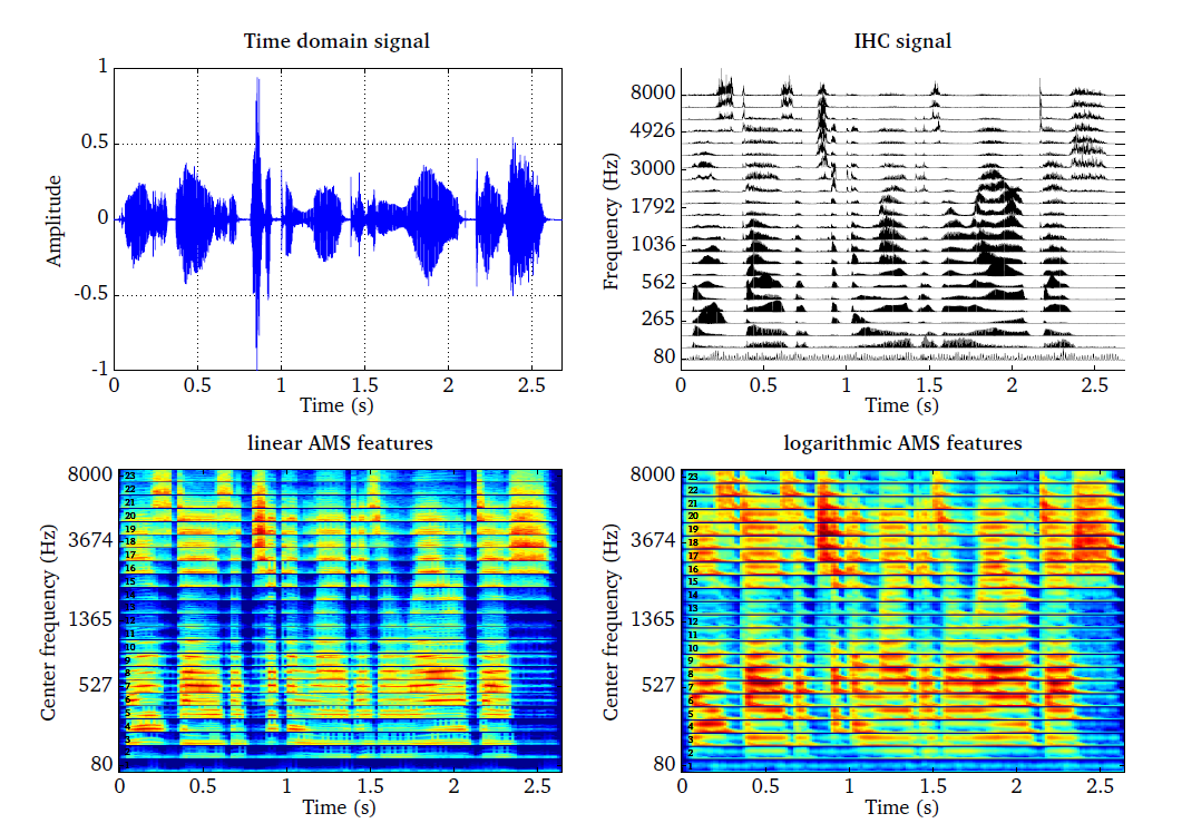
Fig. 21 Speech signal (top left panel) and the corresponding IHC representation (top right panel) using 23 frequency channels spaced between 80 and 8000 Hz. Linear AMS features (bottom left panel) and logarithmic AMS features (bottom right panel). The response of the modulation filters are stacked on top of each other for each IHC frequency channel, and each frequency channel is visually separated by a horizontal black line. The individual frequency channels, ranging from 1 to 23, are labels at the left hand side.
Spectro-temporal modulation spectrogram
Neuro-physiological studies suggest that the response of neurons in the primary auditory cortex of mammals are tuned to specific spectro-temporal patterns [Theunissen2001], [Qiu2003]. This response characteristic of neurons can be described by the so-called STRF. As suggested by [Qiu2003], the STRF can be effectively modelled by two-dimensional (2D) Gabor functions. Based on these findings, a spectro-temporal filter bank consisting of 41 Gabor filters has been designed by [Schaedler2012]. This filter bank has been optimised for the task of ASR, and the respective real parts of the 41 Gabor filters is shown in Fig. 22.
The input is a log-compressed rate-map with a required resolution of 100 Hz, which corresponds to a step size of 10 ms. To reduce the correlation between individual Gabor features and to limit the dimensions of the resulting Gabor feature space, a selection of representative rate-map frequency channels will be automatically performed for each Gabor filter [Schaedler2012]. For instance, the reference implementation based on 23 frequency channels produces a 311 dimensional Gabor feature space.
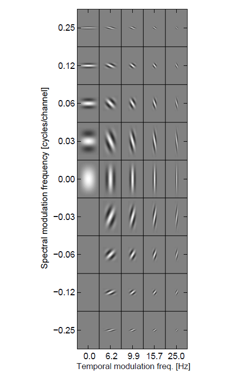
Fig. 22 Real part of 41 spectro-temporal Gabor filters.
The Gabor feature processor is demonstrated by the script
DEMO_GaborFeatures.m, which produces the two plots shown in
Fig. 23. A log-compressed rate-map with 25 ms time frames and 23
frequency channels spaced between 124 and 3657 Hz is shown in the left panel for
a speech signal. These rate-map parameters have been adjusted to meet the
specifications as recommended in the ETSI standard [ETSIES]. The
corresponding Gabor feature space with 311 dimension is presented in the right
panel, where vowel transition (e.g. at time frames around 0.2 s) are well
captured. This aspect might be particularly relevant for the task of ASR.
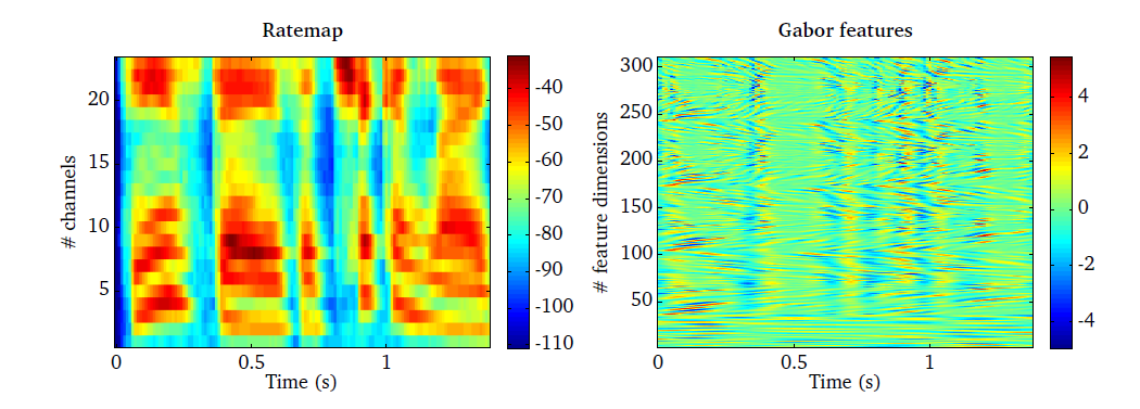
Fig. 23 Rate-map representation of a speech signal (left panel) and the corresponding output of the Gabor feature processor (right panel).
Cross-correlation (crosscorrelationProc.m)
The IHC representations of the left and the right ear signals is used to
compute the normalised CCF in the FFT domain for short time frames of
cc_wSizeSec duration with a step size of cc_hSizeSec. The CCF is
normalised by the auto-correlation sequence at lag zero. This normalised CCF
is then evaluated for time lags within cc_maxDelaySec (e.g., [-1 ms, 1 ms])
and is thus a three-dimensional function of time frame, frequency channel and
lag time. An overview of all CCF parameters is given in
Table 17. Note that the choice of these parameters will
influence the computation of the ITD and the IC processors, which are
described in Interaural time differences (itdProc.m) and Interaural coherence (icProc.m), respectively.
| Parameter | Default | Description |
|---|---|---|
cc_wname |
'hann' |
Window type |
cc_wSizeSec |
0.02 |
Window duration in s |
cc_hSizeSec |
0.01 |
Window step size in s |
cc_maxDelaySec |
0.0011 |
Maximum delay in s considered in CCF computation |
The script DEMO_Crosscorrelation.m demonstrates the functionality of the
CCF function and the resulting plots are shown in Fig. 24. The left
panel shows the ear signals for a speech source that is located closer to the
right ear. As result, the left ear signal is smaller in amplitude and is delayed
in comparison to the right ear signal. The corresponding CCF is shown in the
right panel for 32 auditory channels, where peaks are centred around positive
time lags, indicating that the source is closer to the right ear. This is even
more evident by looking at the SCCF, as shown in the bottom right panel.
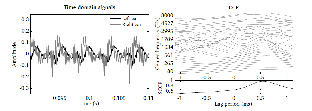
Fig. 24 Left and right ear signals shown for one time frame of 20 ms duration (left panel) and the corresponding CCF (right panel). The SCCF summarises the CCF across all auditory channels (bottom right panel).
Interaural time differences (itdProc.m)
The ITD between the left and the right ear signal is estimated for individual
frequency channels and time frames by locating the time lag that corresponds to
the most prominent peak in the normalised CCF. This estimation is further
refined by a parabolic interpolation stage [May2011], [May2013b]. The ITD
processor does not have any adjustable parameters, but it relies on the CCF
described in Cross-correlation (crosscorrelationProc.m) and its corresponding parameters (see
Table 17). The ITD representation is computed by using
the request entry ’itd’.
The ITD processor is demonstrated by the script DEMO_ITD.m, which produces
two plots as shown in Fig. 25. The ear signals for a speech source
that is located closer to the right ear are shown in the left panel. The
corresponding ITD estimation is presented for each individual TF unit (right
panel). Apart from a few estimation errors, the estimated ITD between both
ears is in the range of 0.5 ms for the majority of TF units.
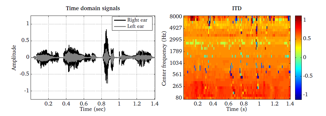
Fig. 25 Binaural speech signal (left panel) and the estimated ITD in ms shown as a function of time frames and frequency channels.
Interaural level differences (ildProc.m)
The ILD is estimated for individual frequency channels by comparing the
frame-based energy of the left and the right-ear IHC representations. The
temporal resolution can be controlled by the frame size ild_wSizeSec and the
step size ild_hSizeSec. Moreover, the window shape can be adjusted by the
parameter ild_wname. The resulting ILD is expressed in dB and negative
values indicate a sound source positioned at the left-hand side, whereas a
positive ILD corresponds to a source located at the right-hand side. A full
list of parameters is shown in Table 18.
| Parameter | Default | Description |
|---|---|---|
ild_wSizeSec |
20E-3 |
Window duration in s |
ild_hSizeSec |
10E-3 |
Window step size in s |
ild_wname |
'hann' |
Window name |
The ILD processor is demonstrated by the script DEMO_ILD.m and the
resulting plots are presented in Fig. 26. The ear signals are shown
for a speech source that is more closely located to the right ear (left panel).
The corresponding ILD estimates are presented for individual TF units. It
is apparent that the change considerably as a function of the centre frequency.
Whereas hardly any ILDs are observed for low frequencies, a strong influence
can be seen at higher frequencies where ILDs can be as high as 30 dB.
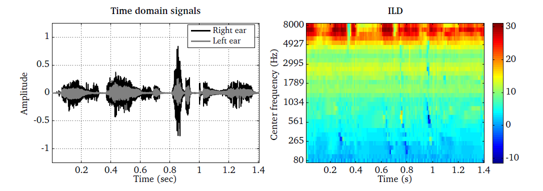
Fig. 26 Binaural speech signal (left panel) and the estimated ILD in dB shown as a function of time frames and frequency channels.
Interaural coherence (icProc.m)
The IC is estimated by determining the maximum value of the normalised CCF.
It has been suggested that the IC can be used to select TF units where the
binaural cues (ITDs and ILDs) are dominated by the direct sound of an
individual sound source, and thus, are likely to reflect the true location of
one of the active sources [Faller2004]. The IC processor does not have any
controllable parameters itself, but it depends on the settings of the CCF
processor, which is described in Cross-correlation (crosscorrelationProc.m). The IC representation is
computed by using the request entry ’ic’.
The application of the IC processor is demonstrated by the script DEMO_IC,
which produces the following four plots shown in Fig. 27. The top left
and bottom left panels show the anechoic and reverberant speech signal,
respectively. It can be seen that the time domain signal is smeared due to the
influence of the reverberation. The IC for the anechoic signal is close to one
for most of the individual TF units, which indicates that the corresponding
binaural cues are reliable. In contrast, the IC for the reverberant signal is
substantially lower for many TF units, suggesting that the corresponding
binaural cues might be unreliable due to the impact of the reverberation.
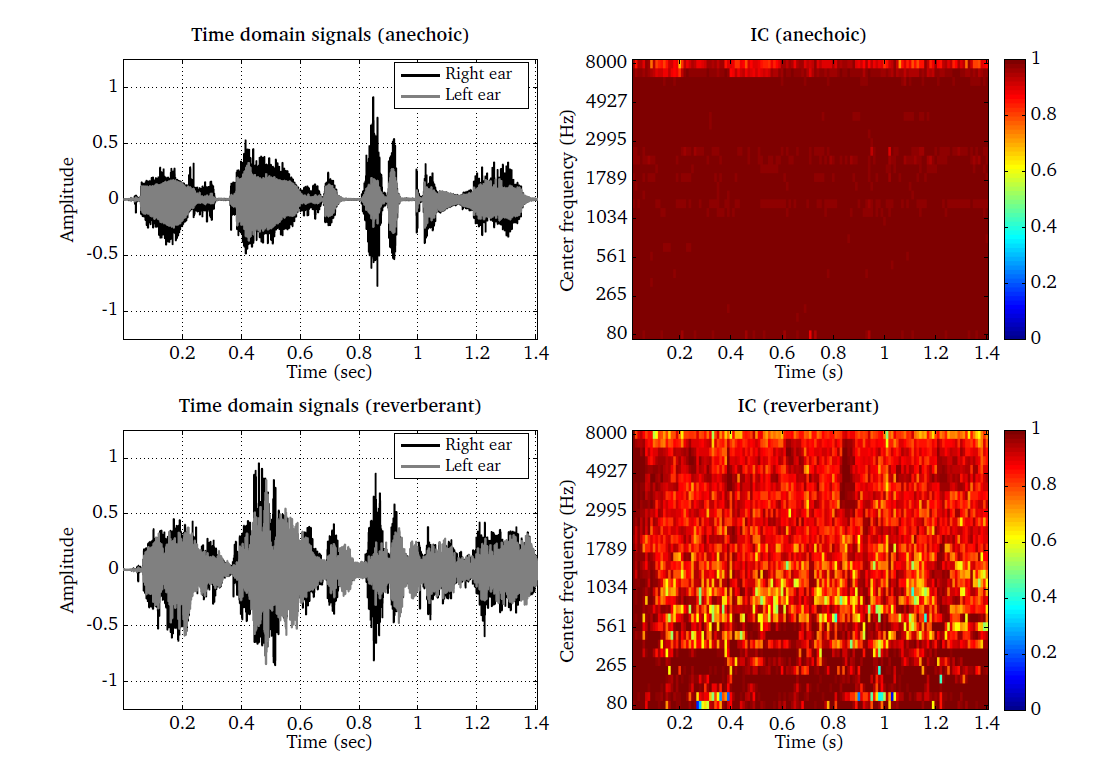
Fig. 27 Time domain signals and the corresponding interaural coherence as a function of time frames and frequency channels estimated for a speech signal in anechoic and reverberant conditions. Anechoic speech (top left panel) and the corresponding IC (top right panel). Reverberant speech (bottom left panel) and the corresponding IC (bottom right panel).
| [Bacon1989] | Bacon, S. P. and Grantham, D. W. (1989), “Modulation masking: Effects of modulation frequency, depths, and phase,” Journal of the Acoustical Society of America 85(6), pp. 2575–2580. |
| [Bernstein1996] | Bernstein, L. R. and Trahiotis, C. (1996), “The normalized correlation: Accounting for binaural detection across center frequency,” Journal of the Acoustical Society of America 100(6), pp. 3774–3784. |
| [Bernstein1999] | (1, 2) Bernstein, L. R., van de Par, S., and Trahiotis, C. (1999), “The normalized interaural correlation: Accounting for NoS thresholds obtained with Gaussian and “low-noise” masking noise,” Journal of the Acoustical Society of America 106(2), pp. 870–876. |
| [Breebart2001] | Breebaart, J., van de Par, S., and Kohlrausch, A. (2001), “Binaural processing model based on contralateral inhibition. I. Model structure,” Journal of the Acoustical Society of America 110(2), pp. 1074–1088. |
| [Bregman1990] | Bregman, A. S. (1990), Auditory scene analysis: The perceptual organization of sound, The MIT Press, Cambridge, MA, USA. |
| [Brown1994] | Brown, G. J. and Cooke, M. P. (1994), “Computational auditory scene analysis,” Computer Speech and Language 8(4), pp. 297–336. |
| [Brown2010] | Brown, G. J., Ferry, R. T., and Meddis, R. (2010), “A computer model of auditory efferent suppression: implications for the recognition of speech in noise.” The Journal of the Acoustical Society of America 127(2), pp. 943–54. |
| [Cooke2001] | Cooke, M., Green, P., Josifovski, L., and Vizinho, A. (2001), “Robust automatic speech recognition with missing and unreliable acoustic data,” Speech Communication 34(3), pp. 267–285. |
| [Dau1996] | (1, 2, 3, 4, 5) Dau, T., Püschel, D., and Kohlrausch, A. (1996), “A quantitative model of the “effective” signal processing in the auditory system. I. Model structure,” Journal of the Acoustical Society of America 99(6), pp. 3615–3622. |
| [Dau1997a] | (1, 2, 3) Dau, T., Püschel, D., and Kohlrausch, A. (1997a), “Modeling auditory processing of amplitude modulation. I. Detection and masking with narrow-band carriers,” Journal of the Acoustical Society of America 102(5), pp. 2892–2905. |
| [Dau1997b] | Dau, T., Püschel, D., and Kohlrausch, A. (1997b), “Modeling auditory processing of amplitude modulation. II. Spectral and temporal integration,” Journal of the Acoustical Society of America 102(5), pp. 2906–2919. |
| [ETSIES] | ETSI ES 201 108 v1.1.3 (2003), “Speech processing, transmission and quality aspects (STQ); distributed speech recognition; front-end feature extraction algorithm; compression algorithms,” URL www.etsi.org. |
| [Ewert2000] | (1, 2) Ewert, S. D. and Dau, T. (2000), “Characterizing frequency selectivity for envelope fluctuations,” Journal of the Acoustical Society of America 108(3), pp. 1181–1196. |
| [Faller2004] | Faller, C. and Merimaa, J. (2004), “Source localization in complex listening situations: Selection of binaural cues based on interaural coherence,” Journal of the Acoustical Society of America 116(5), pp. 3075–3089. |
| [Ferry2007] | Ferry, R. T. and Meddis, R. (2007), “A computer model of medial efferent suppression in the mammalian auditory system,” The Journal of the Acoustical Society of America 122(6), pp. 3519. |
| [Glasberg1990] | (1, 2) Glasberg, B. R. and Moore, B. C. J. (1990), “Derivation of auditory filter shapes from notched-noise data,” Hearing Research 47(1-2), pp. 103–138. |
| [Godde1994] | Goode, R. L., Killion, M., Nakamura, K., and Nishihara, S. (1994), “New knowledge about the function of the human middle ear: development of an improved analog model.” The American journal of otology 15(2), pp. 145–154. |
| [Houtgast1989] | Houtgast, T. (1989), “Frequency selectivity in amplitude-modulation detection,” Journal of the Acoustical Society of America 85(4), pp. 1676–1680. |
| [Jensen2004] | (1, 2, 3, 4) Jensen, K. and Andersen, T. H. (2004), “Real-time beat estimation using feature extraction,” in Computer Music Modeling and Retrieval, edited by U. K. Wiil, Springer, Berlin– Heidelberg, Lecture Notes in Computer Science, pp. 13–22. |
| [Jepsen2008] | (1, 2, 3, 4, 5) Jepsen, M. L., Ewert, S. D., and Dau, T. (2008), “A computational model of human auditory signal processing and perception.” Journal of the Acoustical Society of America 124(1), pp. 422–438. |
| [Joergensen2011] | (1, 2) Jørgensen, S. and Dau, T. (2011), “Predicting speech intelligibility based on the signal-to-noise envelope power ratio after modulation-frequency selective processing,” Journal of the Acoustical Society of America 130(3), pp. 1475–1487. |
| [Joergensen2013] | Jørgensen, S., Ewert, S. D., and Dau, T. (2013), “A multi-resolution envelope-power based model for speech intelligibility,” Journal of the Acoustical Society of America 134(1), pp. 1–11. |
| [Kim2009] | Kim, G., Lu, Y., Hu, Y., and Loizou, P. C. (2009), “An algorithm that improves speech intelligibility in noise for normal-hearing listeners,” Journal of the Acoustical Society of America 126(3), pp. 1486–1494. |
| [Klapuri1999] | Klapuri, A. (1999), “Sound onset detection by applying psychoacoustic knowledge,” in Proceedings of the IEEE International Conference on Acoustics, Speech and Signal Processing (ICASSP), pp. 3089–3092. |
| [Kollmeier1994] | Kollmeier, B. and Koch, R. (1994), “Speech enhancement based on physiological and psychoacoustical models of modulation perception and binaural interaction,” Journal of the Acoustical Society of America 95(3), pp. 1593–1602. |
| [Lerch2012] | (1, 2, 3, 4) Lerch, A. (2012), An Introduction to Audio Content Analysis: Applications in Signal Processing and Music Informatics, John Wiley & Sons, Hoboken, NJ, USA. |
| [Licklider1951] | Licklider, J. C. R. (1951), “A duplex theory of pitch perception,” Experientia (4), pp. 128–134. |
| [Lopez-Poveda2001] | (1, 2, 3) Lopez-Poveda, E. A. and Meddis, R. (2001), “A human nonlinear cochlear filterbank,” Journal of the Acoustical Society of America 110(6), pp. 3107–3118. |
| [May2011] | May, T., van de Par, S., and Kohlrausch, A. (2011), “A probabilistic model for robust localization based on a binaural auditory front-end,” IEEE Transactions on Audio, Speech, and Language Processing 19(1), pp. 1–13. |
| [May2012] | May, T., van de Par, S., and Kohlrausch, A. (2012), “Noise-robust speaker recognition combining missing data techniques and universal background modeling,” IEEE Transactions on Audio, Speech, and Language Processing 20(1), pp. 108–121. |
| [May2013a] | May, T. and Dau, T. (2013), “Environment-aware ideal binary mask estimation using monaural cues,” in IEEE Workshop on Applications of Signal Processing to Audio and Acoustics (WASPAA), pp. 1–4. |
| [May2013b] | May, T., van de Par, S., and Kohlrausch, A. (2013), “Binaural Localization and Detection of Speakers in Complex Acoustic Scenes,” in The technology of binaural listening, edited by J. Blauert, Springer, Berlin–Heidelberg–New York NY, chap. 15, pp. 397–425. |
| [May2014a] | May, T. and Dau, T. (2014), “Requirements for the evaluation of computational speech segregation systems,” Journal of the Acoustical Society of America 136(6), pp. EL398– EL404. |
| [May2014b] | May, T. and Gerkmann, T. (2014), “Generalization of supervised learning for binary mask estimation,” in International Workshop on Acoustic Signal Enhancement, Antibes, France. |
| [May2014c] | May, T. and Dau, T. (2014), “Computational speech segregation based on an auditory-inspired modulation analysis,” Journal of the Acoustical Society of America 136(6), pp. 3350-3359. |
| [Meddis1991] | Meddis, R. and Hewitt, M. J. (1991), “Virtual pitch and phase sensitivity of a computer model of the auditory periphery. I: Pitch identification,” Journal of the Acoustical Society of America 89(6), pp. 2866–2882. |
| [Meddis1997] | Meddis, R. and O’Mard, L. (1997), “A unitary model of pitch perception,” Journal of the Acoustical Society of America 102(3), pp. 1811–1820. |
| [Meddis2001] | (1, 2, 3) Meddis, R., O’Mard, L. P., and Lopez-Poveda, E. A. (2001), “A computational algorithm for computing nonlinear auditory frequency selectivity,” Journal of the Acoustical Society of America 109(6), pp. 2852–2861. |
| [Misra2004] | Misra, H., Ikbal, S., Bourlard, H., and Hermansky, H. (2004), “Spectral entropy based feature for robust ASR,” in Proceedings of the IEEE International Conference on Acoustics, Speech and Signal Processing (ICASSP), pp. 193–196. |
| [Peeters2011] | (1, 2, 3, 4, 5, 6, 7, 8) Peeters, G., Giordano, B. L., Susini, P., Misdariis, N., and McAdams, S. (2011), “The timbre toolbox: Extracting audio descriptors from musical signals.” Journal of the Acoustical Society of America 130(5), pp. 2902–2916. |
| [Pueschel1988] | (1, 2) Püschel, D. (1988), “Prinzipien der zeitlichen Analyse beim Hören,” Ph.D. thesis, University of Göttingen. |
| [Qiu2003] | (1, 2) Qiu, A., Schreiner, C. E., and Escabì, M. A. (2003), “Gabor analysis of auditory midbrain receptive fields: Spectro-temporal and binaural composition.” Journal of Neurophysiology 90(1), pp. 456–476. |
| [Rabiner1977] | Rabiner, L. R. (1977), “On the use of autocorrelation analysis for pitch detection,” IEEE Transactions on Audio, Speech, and Language Processing 25(1), pp. 24–33. |
| [Schaedler2012] | (1, 2) Schädler, M. R., Meyer, B. T., and Kollmeier, B. (2012), “Spectro-temporal modulation subspace-spanning filter bank features for robust automatic speech recognition,” Journal of the Acoustical Society of America 131(5), pp. 4134–4151. |
| [Scheirer1997] | (1, 2) Scheirer, E. and Slaney, M. (1997), “Construction and evaluation of a robust multifeature speech/music discriminator,” in Proceedings of the IEEE International Conference on Acoustics, Speech and Signal Processing (ICASSP), pp. 1331–1334. |
| [Slaney1990] | Slaney, M. and Lyon, R. F. (1990), “A perceptual pitch detector,” in Proceedings of the IEEE International Conference on Acoustics, Speech and Signal Processing (ICASSP), pp. 357–360. |
| [Smith1977] | Smith, R. L. (1977), “Short-term adaptation in single auditory nerve fibers: some poststimulatory effects,” J Neurophysiol 40(5), pp. 1098–1111. |
| [Smith1983] | Smith, R. L., Brachman, M. L., and Goodman, D. a. (1983), “Adaptation in the Auditory Periphery,” Annals of the New York Academy of Sciences 405(1 Cochlear Pros), pp. 79–93. |
| [Soendergaard2013] | (1, 2, 3, 4, 5) Søndergaard, P. L. and Majdak, P. (2013), “The auditory modeling toolbox,” in The Technology of Binaural Listening, edited by J. Blauert, Springer, Heidelberg–New York NY–Dordrecht–London, chap. 2, pp. 33–56. |
| [Tchorz2003] | (1, 2) Tchorz, J. and Kollmeier, B. (2003), “SNR estimation based on amplitude modulation analysis with applications to noise suppression,” IEEE Transactions on Audio, Speech, and Language Processing 11(3), pp. 184–192. |
| [Theunissen2001] | Theunissen, F. E., David, S. V., Singh, N. C., Hsu, A., Vinje, W. E., and Gallant, J. L. (2001), “Estimating spatio-temporal receptive fields of auditory and visual neurons from their responses to natural stimuli,” Network: Computation in Neural Systems 12, pp. 289–316. |
| [Tolonen2000] | (1, 2) Tolonen, T. and Karjalainen, M. (2000), “A computationally efficient multipitch analysis model,” IEEE Transactions on Audio, Speech, and Language Processing 8(6), pp. 708–716. |
| [Turgeon2002] | Turgeon, M., Bregman, A. S., and Ahad, P. A. (2002), “Rhythmic masking release: Contribution of cues for perceptual organization to the cross-spectral fusion of concurrent narrow-band noises,” Journal of the Acoustical Society of America 111(4), pp. 1819–1831. |
| [Tzanetakis2002] | (1, 2) Tzanetakis, G. and Cook, P. (2002), “Musical genre classification of audio signals,” IEEE Transactions on Audio, Speech, and Language Processing 10(5), pp. 293–302. |
| [Wang2006] | Wang, D. L. and Brown, G. J. (Eds.) (2006), Computational Auditory Scene Analysis: Principles, Algorithms and Applications, Wiley / IEEE Press. |
| [Young2006] | Young, S., Evermann, G., Gales, M., Hain, T., Kershaw, D., Liu, X., Moore, G., Odell, J., Ollason, D., Povey, D., Valtchev, V., and Woodland, P. (2006), The HTK Book (for HTK Version 3.4), Cambridge University Engineering Department, URL http://htk.eng.cam.ac.uk. |