Technical description
Introduction
Many different auditory models are available that can transform an input signal into an auditory representation. The actual design challenges behind the Auditory front-end arise from the multiplicity of supported representations, the requirement to process continuous signal in a chunk-based manner, and the ability to change what is being computed at run-time, which will allow the incorporation of feedback from higher processing stages. In addition to these three constraints, the framework will be subject to frequent updates in the future of the Two!Ears project (e.g., adding new processors), so the expandability and maintainability of its implementation should be optimal. For these reasons, the framework is implemented using a modular object-oriented approach.
This chapter exposes the architecture and interactions of all the objects involved in the Auditory front-end and how the main constraints were tackled conceptually. In an effort to respect encapsulation and the hierarchical organisation of the objects, the sections are arranged in a “bottom-up” way: from the most fundamental objects to the more global processes.
All classes involved in the Auditory front-end implementation are inheriting the Matlab
handle master class. This allows every created object to be of the
handle type, and simulates a “call-by-reference” when manipulating the
objects. Given an object obj inheriting the handle class, doing obj2 =
obj will not copy the object, but only obtain a pointer to it. If obj is
modified, then so is obj2. This avoids unnecessary copies of objects,
limiting memory use, as well as providing user friendly handles to objects
included under many levels of class hierarchy. The user can manipulate a simple
short-named handle instead of tediously accessing the object.
Data handling
Circular buffer
Memory pre-allocation of large arrays in Matlab is well known to be a critical operation for optimising computation time. The Auditory front-end, particularly in an online scenario, will be confronted with this problem. For each new chunk of the input signal, chunks of output are computed for each internal representation and are appended to the already existing output. Computation time will be strongly affected if the arrays containing the data are not initialised appropriately (i.e., the memory it occupies is pre-allocated) to fit the input signal duration.
The issue in a real-time scenario is that the signal duration is unknown. To overcome this problem, data for each signal is stored in a buffer of fixed duration which is itself pre-allocated. Buffers are updated following a FIFO rule: once the buffer is full, the oldest samples in the buffer are overwritten by the new signal samples.
The circVBuf class
A conceptual way of implementing a FIFO rule is to use circular (or ring) buffers. The inconvenience of a traditional linear buffer is that once it is full and new input overwrites old samples (i.e., it is in its “steady-state”), reading the data from it implies reaching the end of the buffer and continuing reading from its beginning. The data read will be in two fragments, because of the linear buffer having a physical beginning and end which do not match to the oldest and newest data samples. This is eliminated in circular buffers which do not have a beginning or end, and a contiguous segment is always obtained upon reading. Circular buffers were implemented for the Auditory front-end based on the third-party class provided by [Goebbert2014], which has been slightly modified to account for multi-dimensional data (instead of vector-only).
Circular buffer interface
The circVBuf class provides a buffer that is conceptually circular, in the
sense that it allows continuous reading of the data. However in practice it
still stores data in a linear array in Matlab (the size of which is, however,
twice the size of the actual data). Accessing stored data requires knowledge
about this class and can be tedious to a naive user. To eliminate confusion and
make the buffer transparent to the user, the interface
circVBuffArrayInterface was implemented, with the aim of allowing the buffer
to use most basic array operations.
Given a circular buffer circBuffer, the interface is obtained by
buffer = circVBufArrayInterface(circBuffer)
It will allow the following operations:
buffer(n1:n2)returns stored data between positionsn1andn2, where position1is the oldest sample in the buffer (but not necessarily the first one in the actual array storing data, due to circularity). For multiple dimensions, these indices always refer to the first dimension. To return stored data up to the most recent sample, usebuffer(n1:end).buffer(:)returns all data stored in the buffer (ignoring “empty” sections of the buffer, if said buffer was never filled).buffer(’new’)returns the latest chunk of data that was added to the buffer.length(buffer)returns the effective (i.e., ignoring empty sections) buffer length across its first dimension.size(buffer)returns the effective size of the buffer (including other dimensions).numel(buffer)returns the total number of elements stored (calculated as product of the effective dimensions).isempty(buffer)returnstruewhen no data is stored,falseotherwise.
This provides an array behaviour to the buffers, simplifying greatly their use.
Note
Note that the only limitation is the need of the column
operator : to access all data, as in buffer(:). Without it,
buffer will return a handle to the circVBufArrayInterface
object.
Signal objects
Signals are implemented as objects in the Auditory front-end. To avoid code repetition and make better use of object-oriented concepts, signals are grouped according to their dimensions, as they then share the same properties. The following classes are implemented:
TimeDomainSignalfor one-dimensional (time) signals.TimeFrequencySignalwhich stores two-dimensional signals where the first dimension relates to time (but can be, e.g., a frame index) and the second to the frequency channel. These signals include as an additional property a vector of channel centre frequenciescfHz. Signals of such form are obtained from requesting, for example,’filterbank’,’innerhaircell’,’ild’,... In addition, time-frequency signals containing binary data (used e.g., in onset or offset mapping) have their ownBinaryMasksignal class.CorrelationSignalfor three-dimensional signals where the third dimension is a lag position. These include also thecfHzproperty as well as a vector of lags (lags).ModulationSignalfor three-dimensional signals where the third dimension is a modulation frequency. These includecfHzandmodCfHz(vector of centre modulation frequencies) as properties.FeatureSignalused to store a collection of time-domain signals, each associated to a specific name. Each feature is a single vector, and all of them are arranged as columns of a same matrix. Hence they include an ordered list of features namesfListthat labels each column.
All these classes inherit the parent Signal class. Hence they all
share the following common “read-only” properties:
Label, which is a “formal” description of the signal, e.g.,’Inner hair-cell envelope’, used for example when plotting the signal.Name, which is a name tag unique to each signal type, e.g.,’innerhaircell’. This name corresponds to the name used for a request to the manager.Dimensions, which describes in a short string how dimensions are arranged in the signal, e.g.,’nSamples x nFilters’FsHz, the sampling frequency of this specific signal. If the signal is framed or down-sampled (e.g., like a rate-map or an ILD) this value will be different from the input signal’s sampling frequency.Channel, which states’left’,’right’or’mono’, depending on which channel from the input signal this signal was derived.Data, an interface object (circVBufArrayInterfacedescribed earlier) to the circular buffer containing all data. The actual buffer,Bufis acircVBufobject and a protected property of the signal (not visible to the user).
The Signal class defines the following methods that are then shared
among children objects:
- A super constructor, which sets up the internal buffer according to the signal dimensions. Each children signal class is calling this super constructor before populating its other properties.
- An
appendChunkmethod used to fill the internal buffer. - A
setDatamethod used for initialising the internal buffer given some data. - A
clearDatamethod for re-initialisation. - The
getSignalBlockmethod returning a segment of data of chosen duration, starting from the newest elements. - The
findProcessormethod which, given a handle to a manager object, will retrieve which processor has computed this specific signal (by comparing it with theOutputproperty of each processor, described in General considerations). - A
getParametersmethod which, given a handle to a manager object, will retrieve the list of parameters used in the processing to obtain that signal.
In addition, the Signal class defines an abstract plot method,
which each children should implement. This cannot be defined in the
parent class as the plotting routines will be drastically different
depending on children signal dimensions. Children classes therefore
only implement their own constructor (which still calls the
super-constructor) and their respective plotting routines.
Data objects
Description
Many signal objects are instantiated by the Auditory front-end (one per representation
involved and per channel). To organise and keep track of them, they are
collected in a dataObject class. This class inherits the dynamicprops
Matlab class (itself inheriting the handle) class. This allows to
dynamically define properties of the class.
This way, each signal involved in a given session of the Auditory front-end will be grouped
according to its class in a distinct property of the dataObject, with name
given by the signal signal.Name unique name tag. Extra properties of the
data object include:
bufferSize_swhich is the common duration of allcircVBufobjects in the signals.- A flag
isStereo, which if true will indicate to the data object that all signals come as pairs of left/right channels.
Data objects are constructed by providing an input signal (which can be empty in online scenarios), a mandatory sampling frequency in Hz, a global buffer size (10 s by default), and the number of channels of the input (1 or 2). This number of channel is not necessary if an input signal is used as argument in the constructor but needs to be provided otherwise.
The dataObject definition includes the following, self-explanatory methods:
addSignal(signalToAdd)clearDatagetParameterSummaryreturning a list of all parameters used for the computation of all included signal (given a handle to the corresponding manager).play, provided for user convenience.
Signal organisation
As mentioned before, data objects store signal objects. Each class of signal
occupies a property in the data object named after the signal .Name
property. Multiple signals of the same class will be stored as a cell array in
that property. In the cell array, the first column is always for the left
channel (or mono signal), and the second column for the right channel. If
multiple signals of the same type are present (e.g., if the user requested the
same representation twice but with a change of parameters), then the
corresponding signals are stored in different lines of the array. For instance,
for a session where the user requested the inner hair-cell envelope twice, with
the second request changing only the way of extracting the envelope (i.e., the
parameter ’ihc_method’), the following data object is created:
>> dataObj

dataObj =

  dataObject with properties:

     bufferSize_s: 10
         isStereo: 1
             time: {[1x1 TimeDomainSignal]  [1x1 TimeDomainSignal]}
            input: {[1x1 TimeDomainSignal]  [1x1 TimeDomainSignal]}
        gammatone: {[1x1 TimeFrequencySignal]  [1x1 TimeFrequencySignal]}
    innerhaircell: {2x2 cell}
Each signal-related field except innerhaircell is a cell array of a single
line (one signal), and two columns (for left and right channel). Because the
second request from the user included only a change in parameter for the inner
hair-cell computation, the same initial gammatone signal is used for both,
but there are two output innerhaircell signals (hence a cell array of two
lines) for each channel (hence two columns).
In that case, to distinguish between the two signals and know which one was
computed with which set of parameter, one can call the signal’s
getParameters method. Given a handle to the manager object, it will return a
list of all parameters used to obtain that signal (including parameters used in
intermediate processing steps).
Processors
Processors are at the core of the Auditory front-end. Each processor is responsible for an individual step in the processing, i.e., going from representation A to representation B. They are adapted from existing models documented in the literature such as to allow for block-based (online) processing. This is made possible by keeping track of the information necessary to transition adequately between two chunks of input. The nature of this “information” varies depending on the processor, and we use in the following the term “internal state” of the processor to refer to it. Internal states and online processing compatibility are then assessed in processChunk method and chunk-based compatibility.
A detailed overview of all processors, with a list of all parameters they accept, is given in Available processors. Hence this section will focus on the properties and methods shared among every processors, as well as the techniques employed to make processing compatible with chunk-based inputs.
General considerations
As for signal objects, processors make use of inheritance, with a parent
Processor class. The parent class defines shared properties of the
processor, abstract classes that each children must implement, and a couple of
methods shared among children.
The motivation behind the implementation of these methods is probably not clear at this stage, but should appear in the following sections. Many of these methods are used in the manager object described later for organising and routing the processing such as to always perform as few operations as needed.
Properties
Each processor shares the properties:
Type- describes formally the processing performedInput- list of input signal object handlesOutput- list of output signal object handlesisBinaural- Flag indicating the need of left and right channel as inputFsHzIn- Input signal sampling frequency (Hz)FsHzOut- Output signal sampling frequency (Hz)UpperDependencies- List of processors that directly depend on this processorLowerDependencies- List of processors this processor directly depends onChannel- Audio channel this processor operates onparameters- Parameter object instance that contains parameter values for this processor
These properties are populated automatically when using the Auditory front-end by the manager
class which is described later in Manager. All of them, apart
from Type are implemented as Hidden properties as they should not be
relevant to the user but still need public access by other classes.
In addition, three private properties are implemented:
bHidden- A flag indicating that the processor should be hidden from the framework. This is used for example for “sub-processors” such asdownSamplerProclistenToModify- An event listener for modifications in any lower dependent processorlistenToDelete- An event listener for deletion of any lower dependent processor
Feedback handling
To these two listeners mentioned above correspond two events, hasChanged and
isDeleted. These events are used in connection to feedback as a mean to
communicate between processors. When parameters of a processor are modified, it
will broadcast a message that will be picked up by its upper dependencies which
will then “know” they have to react accordingly (usually by resetting).
Connecting events and listeners is done automatically when instantiating a
“processing tree”. Modifying a parameter is done via the modifyParameter
method which will broadcast the hasChanged message to upper dependencies.
Potentially overridden methods
Most processors behave in similar ways with regard to how many inputs and
outputs they have, as well as how they connect with their dependencies. However,
there can always be exceptions. To provide sufficient code modularity to easily
handle these exceptions without changing existing code, heavy use of methods
overriding was made. This means that general behaviour for a given method is
implemented in the Processor super-class, and any children which needs to
handle things differently will override this specific method. These methods
susceptible to being overridden are the following, in order in which they are
called:
prepareForProcessing: Finalise processor initialisation or re-initialise after receiving feedbackaddInput: Populate theInputpropertyaddOutput: Populate theOutputpropertyinstantiateOutput: Instantiate an output signal and add it to the data objectinitiateProcessing: Calls the processing method, appropriately routing inputs and output signals to the input and output arguments of theprocessChunkmethod.
Any of these method are then overridden in children that do not behave “normally” (e.g., processors with multiple input or outputs)
processChunk method and chunk-based compatibility
General approach
As briefly exposed above, exact computation performed by each processors are taken from published models, and are described individually in Available processors. However, most of the available implementations are for batch processing, i.e., using one whole input signal at once. To be included in the Auditory front-end, these implementations need to be adapted to account for chunk-based processing, i.e., when the input signal is fed to the system in non-overlapping contiguous blocks, or chunks.
Some processors rely on the input only at time t to generate the output at
time t. These processors are then compatible as such with chunk-based
processing. This is the case for instance for the itdProc which given
cross-correlation deduces the . That is because the processor, at time t, is
provided a cross-correlation value as input (which is a function of frequency
and lag), and only locates for each frequency the lag value for which the
cross-correlation is maximal. There is no influence of past (or future) inputs
to provide the output at time t. This is unfortunately not the case for most
processors, which output at a given time will be influenced, to different
extent, by older input. However, so far, all the processing involved in the
Auditory front-end is causal, i.e., might depend on past input, but will not depend on future
input.
Adapting offline implementations to online is of course case-dependent, and how it was done for each individual processors will not be described here. However the same concept is used for each, and can be related to the overlap-save method traditionally used for filtering long signals (or a stream of input signal) with a FIR filter. This concept revolves around using an internal buffer to store the input samples of a given chunk that will influence the processing of the next chunk. Because of the causality, these samples will always be at the end of the present chunk. Considering a processor which is in “steady-state” (i.e., has a populated internal buffer) and a new incoming chunk of input signal, the following steps are performed:
- The buffer is appended in the beginning of the new input chunk. Conceptually, this provides also a chunk of the input signal, but a longer one that starts at an earlier point in time.
- The input extended in this way is processed following the computations described in literature. If the input is required to have specific dimensions in time (e.g., when windowing is performed), then it is virtually truncated to these dimensions (i.e., input samples falling outside the required dimensions are discarded). The goal is for the output to be as long as possible while still being “valid”, i.e., not being influenced by the boundary with the next input chunks. If additional output was generated due to the appended buffer, it is discarded.
- The buffer is updated to prepare for the next input chunk. This step can vary between processors but the idea is to store in the buffer the end of the current chunk which did not generate output, or which will influence the output of next chunk.
An example: rate-map
A practical example to better illustrate the concepts described above is given in the following. The rate-map is conceptually a “framed” version of an IHC multi-channel envelope. The IHC envelope is a two-dimensional representation (time versus frequency), and the rate-map extraction is the same procedure repeated for every frequency channel. Hence the following is described for a single channel. To extract the rate-map, the envelope is windowed by a set of overlapping windows, and its magnitude averaged in each window. This process is adapted to online processing as illustrated in Fig. 6.
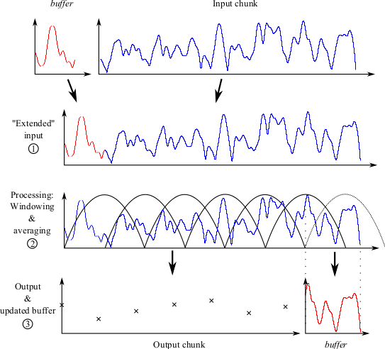
Fig. 6 Three steps for simple online windowing, given a chunk of input and an internal buffer.
The three above-mentioned steps are followed:
- The internal buffer (which can be empty, e.g., if first chunk) is appended to the input chunk.
- This “extended” input is then processed. In that case, it is windowed and the average is taken in each window.
- The “valid” outputs form the output chunk. Note that the right-most window (dashed line) is not fully covering the signal. Hence the output it would provide is not “valid”, since it would also partly depend on the content of the next input chunk. Therefore the section of the signal corresponding to this incomplete window forms the new buffer.
Note that the output chunk could in theory be empty. If the duration of the “extended” input in step 1 is shorter than the duration of the window, then no valid output is produced for this chunk, and the whole extended input will be transferred to the internal buffer. This is unlikely to happen in practice however.
Particular case for filters
The processing performed by the Auditory front-end often involves filtering (e.g., in auditory filter bank processing, inner hair cell envelope detection, or amplitude modulation detection). While filtering by FIR filters could in principle be made compatible with chunk-based processing using the principle described above, it will be impractical for filters with long impulse response, and in theory impossible for IIR filters.
For this reason, chunk-based compatibility is managed differently for filtering.
In Matlab’s filter function, the user can specify initial conditions and can
get as optional output the final conditions of the filter delays. These take the
form of a vector, of dimension equal to the filter order.
In the Auditory front-end, filters are implemented as objects, and encapsulate a private
states property. This property simply contains the final conditions of the
filter delays, i.e., its internal states after the last processing it performed.
If applied to a new input chunk, these states are used as initial condition and
are updated after the processing. This will provide a continuous output given a
fragmented input.
Manager
The manager class is fundamental in the Auditory front-end. It is responsible for, from a
user request, instantiating the correct processors and signal objects, and
linking these signals as inputs/outputs of each processor. In a standard session
of the Auditory front-end, only a single instance of this class is created. It is with this
object that the user interacts.
Processors and signals instantiation
Single request
A standard call to the manager constructor, i.e., with no other argument than a
handle to an already created data object dataObj will produce an “empty”
manager:
>> mObj = manager(dataObj)

mObj =

manager with properties:

    Processors: []
     InputList: []
    OutputList: []
           Map: []
          Data: [1x1 dataObject]
Empty properties include a list of processors, of input signals, output signals,
and a mapping vector that provides a processing order. The Data property is
simply a handle to the dataObj object provided for convenience.
Populating these properties is made via the addProcessor method already
described in Computation of an auditory representation. From a given
request and an empty manager, instantiating the adequate processors and signals
is done following these steps:
- Get the list of signals needed to compute the user request, using the
getDependenciesfunction. - Flip this list around such as to have the list starting with
’time’, and ending up with the requested signal. The list then provides the needed signals in the order they should be computed. - Loop over the elements of the list. For each signal on the list:
- Instantiate a corresponding processor (two if stereo signal)
- Instantiate the signal that will contain the output of the processor (two if stereo)
- Add the signal(s) to
dataObj - A handle to the output signal of the previous processor on the
list is stored as the current processor’s input (in
mObj.InputListas well as in the processor’sInputproperty). If it is the first element of the list, this will link to the original time domain signal. - A handle to the newly instantiated signal is stored similarly as output. This handle is stored further for the next element in the loop.
- A handle to the previously instantiated processor is stored in the
current processor’s
Dependenciesproperty (possibly empty if first element of the list).
- Generate a linear mapping (vector of indexes of the processors ordered in increasing processing order).
- Return a handle to the requested signal to the user.
Once addProcessor called, the properties of the manager will have been
populated, e.g.:
>> mObj

mObj =

  manager with properties:

    Processors: {3x2 cell}
     InputList: {3x2 cell}
    OutputList: {3x2 cell}
           Map: [1 2 3]
          Data: [1x1 dataObject]
Processors are arranged with the same convention as for signals in a data objects: they are stored in a cell array, where the first column is for left (or mono) channel, and second column for right channel. Different lines are for different processors, e.g.:
>> mObj.Processors

ans =

    [1x1 preProc      ]    [1x1 preProc      ]
    [1x1 gammatoneProc]    [1x1 gammatoneProc]
    [1x1 ihcProc      ]    [1x1 ihcProc      ]
InputList and OutputList are cell arrays of handles to signal objects.
An element in one of them will correspond to the input/output of the processor
at the same position in the cell array.
Handling of multiple requests
The above-described process gets more complicated when a request is placed in a non-empty manager (i.e., when multiple requests have been placed). The same steps could be used, and would result in a functioning result. However, this would likely be sub-optimal in terms of computations. If the new request has common elements with representations that are already computed, one need not recompute them.
If correctly implemented, a manager should be able to “branch” the processing,
such that only new representations, or representations where a parameter has
been changed, are recomputed. Achieving this relies on the findInitProc
method of the manager, which is described in more details in the next
subsection. This method is passed the same arguments as the addProcessor
method, i.e., a request name and a structure of parameters. It will return a
handle to an already existing processor in the manager that is exactly computing
one of the steps needed for that request. It will return the “highest” already
existing step. In other terms, it finds the point in the already existing
ordered list of processors where the processing should “branch out” to obtain
the newly requested feature. Knowing the processor to start from and updating
accordingly the list of signals/processors that need to be instantiated, the
same procedure as before can then be used in the addProcessor method.
The findInitProc method
To find an initial processor suitable in a request, this method calls the
hasProcessor method of the manager and the hasParameters method of each
processor. From a given request, it can obtain a list of necessary processing
steps from getDependencies and run the list backwards. For each element of
the list, findInitProc “asks” the manager if it has such a processor via its
hasProcessor method. If yes, it calls this processor hasParameters
method to verify that what the processor computes corresponds to the request. If
yes, then it found a suitable initial step. If no, it moves on to the next
element in the list and repeats.
Carrying out the processing
As of the current Auditory front-end implementation, the processing is linear and the
processChunk methods of each individual processor are called one after the
other when asking the manager to start processing (either via its
processChunk or processSignal method). The order in which the processors
are called is important, as some will take as input what was other’s output.
This order is stored in the property Map of the manager. Map is a vector
of indexes corresponding to the lines in the Processors cell array property
of the manager. It is constructed at instantiation of the processors.
Conceptually, if there are N instantiated processors, the processChunk
method of the manager mObj will call the processChunk methods of each
processor following this loop:
for ii = 1 : N
    % Get index of current processor
    jj = mObj.Map(ii);

    % Getting input signal handle (for code readability)
    in = mObj.InputList{jj,1};

    % Perform the processing
    out = mObj.Processors{jj,1}.processChunk(in.Data('new'));

    % Store the result
    mObj.OutputList{jj,1}.appendChunk(out);
end
Note
Note the difference between indexes ii which relate to the
processing order (processing first ii=1 and last ii=N) and
jj = mObj.Map(ii) which relate the processing order with the actual
position of the processors in the cell array mObj.Processors.
| [Goebbert2014] | Göbbert, J. H. (2014), “Circular double buffered vector buffer (circVBuf.m),” Matlab file exchange: http://www.mathworks.com/matlabcentral/fileexchange/47025-circvbuf, accessed: 2014-10-30. |