openAFE, a C++ library for rosAFE
openAFE is an independant, open-source, library providing the core
algorithmic functionalities needed by the ROS implementation of the genuine
Matlab Auditory front-end. It is written in C++ and implements the extraction of a subset
of common auditory representations from an offline binaural recording, or
from a real- time stream of binaural audio data.
Installation
Note
For all the following installation instructions, we will assume that you are
using a Ubuntu GNU/Linux as it is the supported distribution for ROS. Even
if openAFE does not exploit any ROS capabilities, this library is
mandatory for the actual rosAFE implementation, thus justifying this
requirement. All the guidelines here have been successfully tested on the
14.04 LTS version of Ubuntu.
openAFE links against existing two external libraries:
the BOOST library which is a set of over 80 individual C++ libraries providing everything needed to perform linear algebra, multithreading, image processing, etc. computations.
openAFEexploits its circular buffer implementation to represent audio signal buffers. It can be installed with$ sudo apt-get install libboost1.54-all-dev
the FFTW library; FFTW is among the fastest implementation of the Fast Fourier transform and is widely used when dealing with signal frequency representations. It can be installed with
$ sudo apt-get install lib-fftw3-dev
openAFE can be installed with or without demos, which require a Matlab
installation. Whatever your choice, you will have to get first the
openAFE repository in your home folder (you can choose another location,
but we recommend this one):
$ cd
$ git clone https://github.com/TWOEARS/openAFE
Now, go inside the newly cloned repository, and create the build folder:
$ cd  openAFE
$ mkdir  build
$ cd  build
Standalone version
If you are interested in the installation of a standalon version of
openAFE, without any demo binaries, you have then to use the following
commands inside the build folder:
$ ../configure
$ make
$ sudo make install
The library libopenAFE.so is then installed in /usr/local/lib, while
the header files are in the /usr/local/include/openafe/ folder.
Complete version, with demo binaries
If you are interested in the installation of the complete version of
openAFE, including all demo binaries, you have then to use the following
commands inside the build folder:
$ ../configure  LDFLAGS="-L/usr/local/MATLAB/R2015b/bin/glnxa64" CPPFLAGS="-I/usr/local/MATLAB/R2015b/extern/include  -Wl,-rpath=/usr/local/MATLAB/R2015b/bin/glnxa64"
$ make
$ sudo make install
Note
Depending on your Matlab installation, the paths used during the configure
step above must be changed accordingly. Note also that the installation of
the complete version is optional. The demos are only provided to test and
ilustrate use cases of the openAFE library. The rosAFE component
does not require them.
The library libopenAFE.so is then installed in /usr/local/lib,
the demo binaries can be found in /usr/local/bin, while
the header files are in the /usr/local/include/openafe/ folder.
Demos
openAFE contains a demo binary per processor type. The source code of
these examples can be found in the examples folder of the repository. Each
binary takes a .mat file as input, which must contains an matrix
earSignals of size M samples x 2 corresponding to the binaural
input signal, and a scallar fsHz corresponding to the sampling frequency.
In the same vein, the binary create a .mat file as well as output. This
file contains the data in two separate matrices (left and right channels), and
a value called fsHz which is the sampling frequency.
Note
Three .mat are provided as examples in the examples/Test_signals/
folder of the repository. They all can be used as input to the demo binaries.
For each demo, you should provide at least the following arguments:
inFilePath: the path of the input.matfileoutputName: the name of the output.matfile (including the.matextension)- All other arguments (parameters of the processors) are optional. If missing, default values will be used.
Importantly, all the processors that have to be created to compute the requested audio representation are initialized with their default parameters. As an example, the following code can be used to test the gammatone filterbank processor directy from a terminal:
$ DEMO_filterbank inFilePath outputName fb_lowFreqHz fb_highFreqHz fb_nERBs fb_nChannels fb_nGamma fb_bwERBs
where the arguments are:
fb_lowFreqHz: lowest center frequencyfb_highFreqHz: highest center frequencyfb_nERBs: distance between neighboring filters in ERBsfb_nChannels: channels center frequencies (Hz)fb_nGamma: gammatone rising slope orderfb_bwERBs: bandwidth of the filters in ERBs
You can notice that these arguments are identical to those of the Matlab
Auditory front-end. This will be the case for all the processors implemented in
openAFE (see below).
Implementation details
Signal representation
Input or output signals are described through standard C++ classes defining
attributes and methods for their parameterization, creation and destruction.
At first, a general openAFE::Signal class is defined, highlighting common
attributes and methods inherited by the more specific signal classes described
in the following. For instance, a signal instance is represented by its name,
its sampling frequency, the channel it represents (mono, left or right
channel) and its size.
All signal instances share the same signal buffer description, relying on the
Boost.CircularBuffer class provided by the BOOST library. Data inside a
circular buffer can be accessed by requiring the whole buffer, only the last
appended chunk, only last appended N frames, or the whole new frames, through
the corresponding methods getWholeBufferAccesor(),
getLastChunckAccessor(), getLastDataAccessor() and
getOldDataAccessor() respectively.
On this basis, three dedicated signal classes are defined, both of them
inheriting from the general openAFE::Signal class (see the inheritance
diagram Fig. 7). These three signal classes directly
reproduce the signal definitions from the genuine Matlab Auditory front-end (see
the signal objects definitions from the Matlab
AFE), namely:
openAFE::TimeDomainSignal, for one-dimensional (time) signals,openAFE::TimeFrequencySignal, which corresponds to two-dimensional signals, with the first dimension related to time and the second to the frequency channel,openAFE::CorrelationSignal, for three-dimensional signals where the third dimension is a lag position.
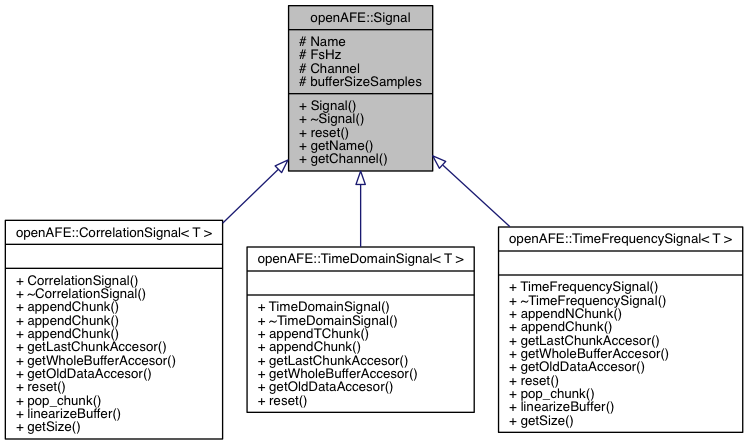
Fig. 7 Inheritance diagram for the openAFE::Signal class.
Processor representation
Processors are responsible for one individual step in the extraction of a
given audio representation. In the Matlab Auditory front-end implementation, processors are
connected to each other, thus forming a tree: a processor whose output is
routed to another processor’s input is henceforth called parent while the
second one is called child. Of course, a processor can have multiple
children, and multiple parents as well. openAFE implementation of
processors is still rooted on this tree architecture.
Data exchange between processors
The tree workflow has been implemented through an object oriented description, providing general methods to access data from a parent processor, process it, and release it to its child(ren). Basically, each processor instantiation contains a pointer to his parent(s), but does not include any information about his own child(ren). Therefore, the data flow between two processors are handled by two general methods:
processChunk(), which gets data from the parent processor and process it. Once the representation is obtained, the result is stored on a private internal memory zone (the attributesleftPMZandrightPMZ), ready to be used by its child(ren);- Then,
releaseChunk()can be used to search for the last chunk of data available in this private memory zone, and to append it to the output signal of the processor.
Such an approach avoids each child of a processor to make a local copy of their parent output(s), which then shares a read access to its own output. This way, the shared resource is not replicated for each child(ren), thus limiting the memory needs.
Processor classes description
Multiple classes have been used to describe all processors. On the top of all
representations is the openAFE::Processor class, which describes the
general common properties and methods of all processors. This includes the
aforementioned chunk processing methods processChunk() and
releaseChunk(), but also attributes like the name of the processor, its
sampling frequency, its input and output size, etc. On this basis, three
classes are inheriting this description, each of them being dedicated to time-
based, frequency-based and lag-based processors. This is to put in parallel
to the three aforementionned signal classes openAFE::TimeDomainSignal (1D
signals), openAFE::TimeFrequencySignal (2D signals) and
openAFE::CorrelationSignal (3D signals). Each of them gives rise to
specific processor classes, which actually implements the processors
representation (see the inheritance diagram Fig. 8).
For now, the 7 available processors are listed in Table 5.
| Type | Name |
|---|---|
| Processors | Input Processor |
| Pre-Processor (DC removal filter, Pre-emphasis filter, Binaural RMS normalization, Level scaling) | |
| Filterbank (Gammatone) | |
| Inner Hair Cell (Methods : none, halfwave, fullwave, square, dau) | |
| Interaural Level Difference (Windows : hamming, hann, blackman, triangular, square root) | |
| Ratemap (Windows : hamming, hann, blackman, triangular, square root) | |
| Cross-Correlation |
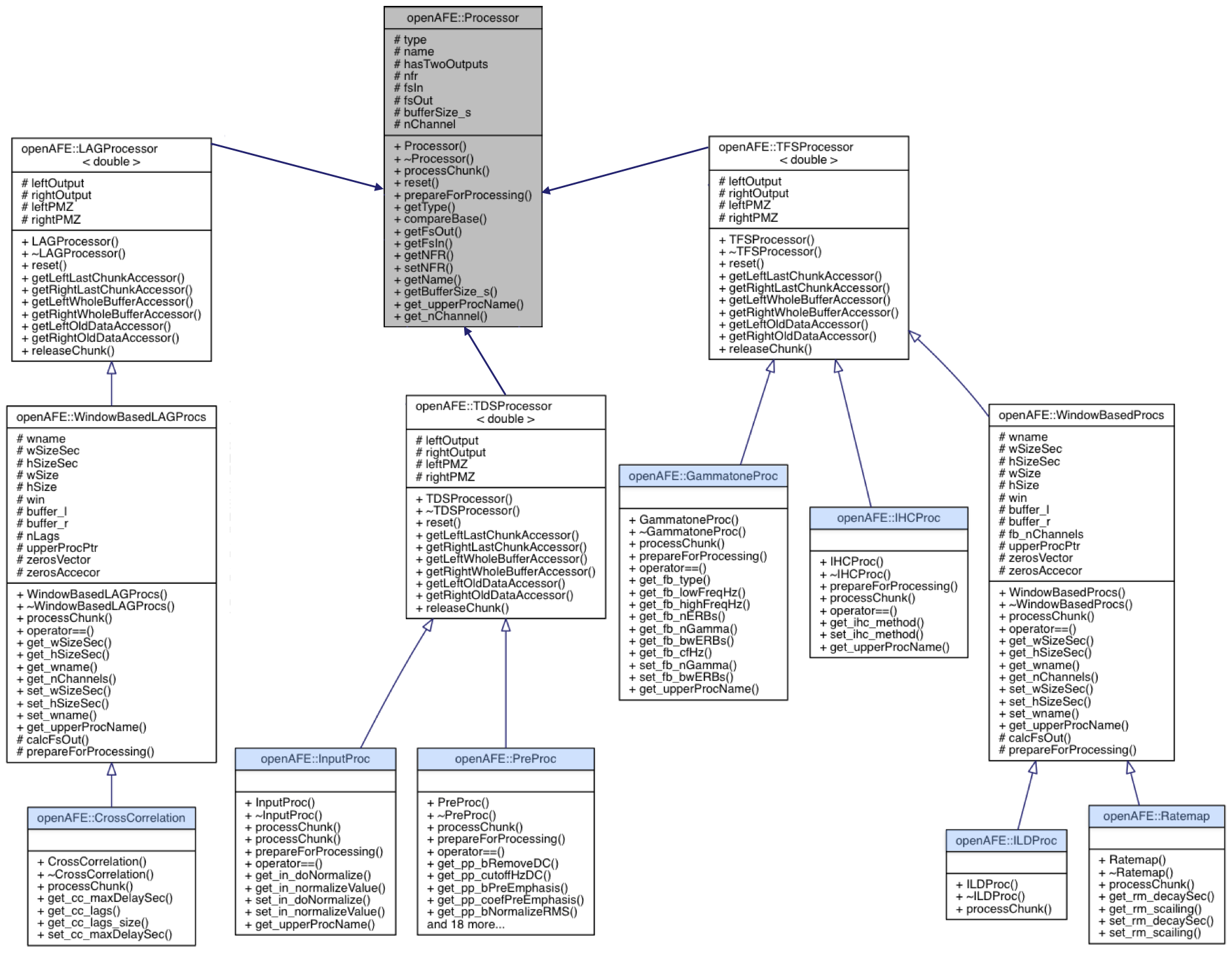
Fig. 8 Inheritance diagram for the openAFE::Processor class.
Processor parameters
All the processor parameters, which all appear as attributes of their corresponding classes, are absolutely identical to the genuine Matlab processor implementation (see here for a comprehensive list).
Note that any change in a processor parameter may require some preparation
before being actually used in the processing: for instance, changing the cut-
off-frequency of a filter yields to the re-initialization of this filter. This
preparation must be explicitly called after a change of parameter through the
corresponding prepareForProcessing() method. Note also that each parameter
is coupled with corresponding set() and get() methods, which allow to
respectively set or read the parameter value of the instantiated processor.
Except the blacklisted parameters listed in the original AFE, all the
parameters can be modified at any time, thus allowing top-down feedback from
higher levels of the Two!Ears architecture. The new parameters are
immediately used for the new chunks arriving just after the modification.
Code example
The following C++ code shows how the openAFE library can be used to
compute the gammatone filterbank outputs from a binaural signal recorded
inside a .mat file. This also illustrates the processing scheme explained
above, using the processChunk() and releaseChunk() methods. This
example exploits some additional code to be able to read and write from/to
.mat files. This code has been compiled to form a library
libmatFiles.a during the openAFE installation (the library and its
header file are located in the build/example folder). The example below
must be then linked against this library to correctly operate. This
requirement can be relaxed when working directly on data structures defined in
the code.
To compile the example, first download the example source code file to the ~/TEST folder, and follow the steps below:
$ cd TEST
$ cp ../openAFE/examples/matFiles.hpp .
$ cp ../openAFE/build/examples/libmatFiles.a .
$ cp ../openAFE/examples/Text_signals/DEMO_Speech_Anechoic.mat .
$ sed -i -e 's/..\/src\/Signals\/dataType.hpp/Signals\/dataType.hpp/g' matFiles.hpp
$ g++ -Wall -O3 -std=c++11 -pthread -Wl,-rpath=/usr/local/MATLAB/R2015b/bin/glnxa64 -I/usr/local/include/openafe -I/usr/local/MATLAB/R2015b/extern/include -L/usr/local/MATLAB/R2015b/bin/glnxa64 test.cpp -o test -lopenAFE libmatFiles.a -lmat -lmx -lm
You then get a binary file test, which can be run directly from the command line:
$ ./test
The example reads the data from the DEMO_Speech_Anechoic.mat, process it,
and writes the output to a out.mat file. The source code of the example is
reproduced here:
#include <memory>
#include <iostream>

#include "matFiles.hpp"
#include "openafe/Processors/inputProc.hpp"
#include "openafe/Processors/preProc.hpp"
#include "openafe/Processors/gammatoneProc.hpp"

using namespace openAFE;
using namespace std;

int main(int argc, char **argv) {

  // Read input from .mat file
  string dataPath("./DEMO_Speech_Anechoic.mat");
  vector <vector<double> > earSignals;
  double fsHz;
  matFiles::readMatFile(dataPath.c_str(), earSignals, &fsHz);

  // Gammaton processor parameters
  filterBankType fb_type = _gammatoneFilterBank;
  double fb_lowFreqHz = 80;
  double fb_highFreqHz = 8000;
  double fb_nERBs = 1;
  uint32_t fb_nChannels = 0;
  double* fb_cfHz = nullptr;
  size_t fb_cfHz_length = 0;
  uint32_t fb_nGamma = 4;
  double fb_bwERBs = 1.0180;

  /// Processor instanciations
  // Input processor
  shared_ptr <InputProc > inputP;
  inputP.reset( new InputProc("input", fsHz, 10 /* bufferSize_s */, false /* doNormalize */) );

  // Pre-processor
  shared_ptr <PreProc > ppP;
  ppP.reset( new PreProc("preProc", inputP ) ); /* default parameters */

  // Gammatone processor
  shared_ptr <GammatoneProc > gtP;
  gtP.reset( new GammatoneProc("gammatoneProc", ppP ,fb_type,
                                fb_lowFreqHz,
                                fb_highFreqHz,
                                fb_nERBs,
                                fb_nChannels,
                                fb_cfHz,
                                fb_cfHz_length,
                                fb_nGamma,
                                fb_bwERBs ) );

  /// Successive computations in the tree to obtain the required audio representation
  // First, input Processor
  inputP->processChunk ( earSignals[0].data(), earSignals[0].size(), earSignals[1].data(), earSignals[1].size() );
  inputP->releaseChunk();

  // Then the pre-Processor
  ppP->processChunk ();
  ppP->releaseChunk();

  // And finally, the gammatone Processor
  gtP->processChunk ();
  gtP->releaseChunk();

  /// Outputs are in the lOut and rOut variables
  vector<shared_ptr<twoCTypeBlock<double> > > lOut = gtP->getLeftWholeBufferAccessor();
  vector<shared_ptr<twoCTypeBlock<double> > > rOut = gtP->getRightWholeBufferAccessor();

  // Eventually, write the signals into a .mat file
  matFiles::writeTFSMatFile("out.mat", lOut, rOut, fsHz);


}