Identification of sound types
This example particularly serves to demonstrate two aspects of the Two!Ears Auditory Model:
- Building a Blackboard system dynamically in code (instead of via xml definition, as demonstrated in the Localisation with and without head rotations example)
- Using identity knowledge sources with source type models to generate hypotheses about the type of sound objects in an auditory scene.
The base folder for this example is examples/identification, with the
main example script file being identify.m. Other than that, there is the
file SceneDescription.xml which describes the Binaural simulator configuration.
A directory models/test_1vsAll_training contains files which hold the source type models used in this example, a sound file list
shortTest.flist, and subfunctions (buildIdentificationBBS.m,
makeTestSignal.m, setDefaultIdModels.m) used in
identify.m. Have a look at
Train sound type identification models to see how the source type models have
been created. To see if everything is working, just run
>> identify;
Example step-through
To dive into the example, load up Matlab, navigate into the example directory,
and open identify.m, which contains a function (also usable as a
script without arguments). Let’s have a look before firing it up!
Specifying the identification models
The function identify takes a parameter, which shall specify the models to
be used for source type identification. However, for this example, you can run
without setting this parameter, and let the function setDefaultIdModels do
this for you.
if nargin < 1, idModels = setDefaultIdModels(); end
This function specifies six source type models by giving the directories they are located in and the class they are trained to identify, respectively.
Creating a test scene
To test the identification models, a test scene is compiled from audio events
(IEEE AASP single event sounds database) from several
wav-files, listed in shortTest.flist. All those wav-files have not been
used for training of the tested models (the models have all been trained using the
same trainset), so the models have never “seen” (or better: “heard”) these
actual sounds. The function makeTestSignal not only compiles the audio, but
also reads the “ground truth”, i.e. the on- and offset times of the respective
events from the annotation files. The scene is about 45 seconds long. The events
are concatenated in random order (with 0.5s inbetween two events).
Initialising the Binaural Simulator
The next code paragraph deals with initialisation of the Binaural simulator. More
specific, the acoustic sources are set to a head-relative azimuth of zero
degrees and three meters distance. Free-field conditions (no reverberation) are
set through absence of a room definition (either in the
SceneDescription.xml or in code). The models have been trained under the
same conditions.
Building the example Blackboard System
The construction of the Blackboard system for this example is done directly in Matlab
(versus via xml) in the function buildIdentificationBBS. Let’s look into it,
we first create a new BlackboardSystem object:
bbs = BlackboardSystem(1);
This object is our access point and frame for the simulation. We first set up the connection to the Binaural simulator and the Auditory front-end:
bbs.setRobotConnect(sim);
bbs.setDataConnect('AuditoryFrontEndKS');
Followed by invocation of the identity knowledge sources using the function createKS of the
Blackboard system, which also takes care to place the Auditory front-end requests at
the AuditoryFrontEndKs. The identity knowledge
sources need name and location of the source type models they load and represent
in the system. The third argument serves as a preprocessing flag for removing the DC component from the ear signals.
We set the invocation frequency of the knowledge sources to 100ms (default value is
250ms):
for ii = 1 : numel( idModels )
    idKss{ii} = bbs.createKS('IdentityKS', {idModels(ii).name, idModels(ii).dir, ppRemoveDc});
    idKss{ii}.setInvocationFrequency(10);
end
We create one more knowledge source, the IdTruthPlotKS – it’s not really a knowledge source in the sense of the word in this case, but a handy way to implement a debugging tool for live-inspection of the identity information in the blackboard system. It needs the ground truth information passed to it:
idCheat = bbs.createKS('IdTruthPlotKS', {labels, onOffsets});
In the last lines dealing with blackboard system construction, we connect the different modules:
bbs.blackboardMonitor.bind({bbs.scheduler}, {bbs.dataConnect}, 'replaceOld', 'AgendaEmpty' );
bbs.blackboardMonitor.bind({bbs.dataConnect}, idKss, 'replaceOld' );
bbs.blackboardMonitor.bind(idKss, {idCheat}, 'replaceParallelOld' );
- The
dataConnectgets bound to the scheduler – this way, the next chunk of acoustic data is fetched whenever no more knowledge source needs to be processed - The identity knowledge sources get bound to the
dataConnect(which we have instantiated to be the AuditoryFrontEndKS before) - The
IdTruthPlotKSgets bound to the identity knowledge sources, which produce the identity hypotheses.
Running the simulation
With the blackboard system set up, we can start the simulation,
bbs.run();
which will trigger the first fetching of acoustic data by the system, followed by processing and triggering subsequent events and knowledge source executions. The blackboard system is set up to “verbose” mode, printing the events and executions on the Matlab console:
-------- [Event Fired:] Scheduler -> (AgendaEmpty) -> AuditoryFrontEndKS
-------- [Executing KS:] AuditoryFrontEndKS
-------- [Event Fired:] AuditoryFrontEndKS -> (KsFiredEvent) -> IdentityKS[clearthroat]
-------- [Event Fired:] AuditoryFrontEndKS -> (KsFiredEvent) -> IdentityKS[knock]
-------- [Event Fired:] AuditoryFrontEndKS -> (KsFiredEvent) -> IdentityKS[switch]
-------- [Event Fired:] AuditoryFrontEndKS -> (KsFiredEvent) -> IdentityKS[keyboard]
-------- [Event Fired:] AuditoryFrontEndKS -> (KsFiredEvent) -> IdentityKS[speech]
-------- [Executing KS:] IdTruthPlotKS
-------- [Executing KS:] IdentityKS[clearthroat]
....Identity Hypothesis: clearthroat with 75% probability.
-------- [Event Fired:] IdentityKS[clearthroat] -> (KsFiredEvent) -> IdTruthPlotKS
-------- [Executing KS:] IdentityKS[knock]
....Identity Hypothesis: knock with 0% probability.
-------- [Event Fired:] IdentityKS[knock] -> (KsFiredEvent) -> IdTruthPlotKS
-------- [Executing KS:] IdentityKS[switch]
....Identity Hypothesis: switch with 6% probability.
-------- [Event Fired:] IdentityKS[switch] -> (KsFiredEvent) -> IdTruthPlotKS
-------- [Executing KS:] IdentityKS[keyboard]
....Identity Hypothesis: keyboard with 0% probability.
-------- [Event Fired:] IdentityKS[keyboard] -> (KsFiredEvent) -> IdTruthPlotKS
-------- [Executing KS:] IdentityKS[speech]
....Identity Hypothesis: speech with 89% probability.
-------- [Event Fired:] IdentityKS[speech] -> (KsFiredEvent) -> IdTruthPlotKS
You can see the before installed event bindings in action – the scheduler triggers the AuditoryFrontEndKS, which triggers the IdentityKSs, which place identity hypotheses on the blackboard and trigger the IdTruthPlotKS.
The simulation will take a few minutes – as mentioned, it processes a 45s scene, and at the moment, is not optimised to run in real-time. You can see the progress in the id truth plot, which shows the wave form of the left channel (ear) accompanied by a graphical representation of the events, ground truth versus hypotheses produced by the models:
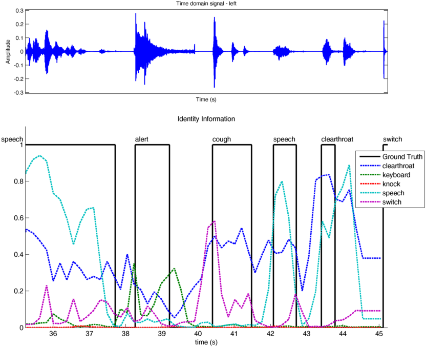
Fig. 76 This is the live plot of hypotheses created by the identity knowledge sources, in comparison to the “ground truth” (as given by annotated on- and offset times for the source sound files).
Evaluating the simulation
Finally, idScoresRelativeError calculates an error rate of the tested models
for this example:
Evaluate scores...

relative error of clearthroat identification model: 0.244339
relative error of keyboard identification model: 0.112274
relative error of knock identification model: 0.034251
relative error of speech identification model: 0.095172
relative error of switch identification model: 0.110843
The relative error rate here is the over time integrated difference between ground truth and model hypotheses (divided by the length of the simulation).