Spectral features (spectralFeaturesProc.m)
In order to characterise the spectral content of the ear signals, a set of spectral features is available that can serve as a physical correlate to perceptual attributes, such as timbre and coloration [Peeters2011]. All spectral features summarise the spectral content of the rate-map representation across auditory filters and are computed for individual time frames. The following 14 spectral features are available:
'centroid': The spectral centroid represents the centre of gravity of the rate-map and is one of the most frequently-used timbre parameters [Tzanetakis2002], [Jensen2004], [Peeters2011]. The centroid is normalised by the highest rate-map centre frequency to reduce the influence of the gammatone parameters.'spread': The spectral spread describes the average deviation of the rate-map around its centroid, which is commonly associated with the bandwidth of the signal. Noise-like signals have usually a large spectral spread, while individual tonal sounds with isolated peaks will result in a low spectral spread. Similar to the centroid, the spectral spread is normalised by the highest rate-map centre frequency, such that the feature value ranges between zero and one.'brightness': The brightness reflects the amount of high frequency information and is measured by relating the energy above a pre-defined cutoff frequency to the total energy. This cutoff frequency is set tosf_br_cf = 1500Hz by default [Jensen2004], [Peeters2011]. This feature might be used to quantify the sensation of sharpness.'high-frequency content': The high-frequency content is another metric that measures the energy associated with high frequencies. It is derived by weighting each channel in the rate-map by its squared centre frequency and integrating this representation across all frequency channels [Jensen2004]. To reduce the sensitivity of this feature to the overall signal level, the high-frequency content feature is normalised by the rate-map integrated across-frequency.'crest': The SCM is defined as the ratio between the maximum value and the arithmetic mean and can be used to characterise the peakiness of the rate-map. The feature value is low for signals with a flat spectrum and high for a rate-map with a distinct spectral peak [Peeters2011], [Lerch2012].'decrease': The spectral decrease describes the average spectral slope of the rate-map representation, putting a stronger emphasis on the low frequencies [Peeters2011].'entropy': The entropy can be used to capture the peakiness of the spectral representation [Misra2004]. The resulting feature is low for a rate-map with many distinct spectral peaks and high for a flat rate-map spectrum.'flatness': The SFM is defined as the ratio of the geometric mean to the arithmetic mean and can be used to distinguish between harmonic (SFM is close to zero) and a noisy signals (SFM is close to one) [Peeters2011].'irregularity': The spectral irregularity quantifies the variations of the logarithmically-scaled rate-map across frequencies [Jensen2004].'kurtosis': The excess kurtosis measures whether the spectrum can be characterised by a Gaussian distribution [Lerch2012]. This feature will be zero for a Gaussian distribution.'skewness': The spectral skewness measures the symmetry of the spectrum around its arithmetic mean [Lerch2012]. The feature will be zero for silent segments and high for voiced speech where substantial energy is present around the fundamental frequency.'roll-off': Determines the frequency in Hz below which a pre-defined percentagesf_ro_percof the total spectral energy is concentrated. Common values for this threshold are betweensf_ro_perc = 0.85[Tzanetakis2002] andsf_ro_perc = 0.95[Scheirer1997], [Peeters2011]. The roll-off feature is normalised by the highest rate-map centre frequency and ranges between zero and one. This feature can be useful to distinguish voiced from unvoiced signals.'flux': The spectral flux evaluates the temporal variation of the logarithmically-scaled rate-map across adjacent frames [Lerch2012]. It has been suggested to be useful for the distinction of music and speech signals, since music has a higher rate of change [Scheirer1997].'variation': The spectral variation is defined as one minus the normalised correlation between two adjacent time frames of the rate-map [Peeters2011].
A list of all parameters is presented in Table 25.
| Parameter | Default | Description |
|---|---|---|
sf_requests |
'all' |
List of requested spectral features (e.g.
to display the full list of supported spectral features. |
sf_br_cf |
1500 |
Cut-off frequency in Hz for brightness feature |
sf_ro_perc |
0.85 |
Threshold (re. 1) for spectral roll-off feature |
The extraction of spectral features is demonstrated by the script
Demo_SpectralFeatures.m, which produces the plots shown in
Fig. 27. The complete set of 14 spectral features is
computed for the speech signal shown in the top left panel. Whenever the unit of
the spectral feature was given in frequency, the feature is shown in black in
combination with the corresponding rate-map representation.
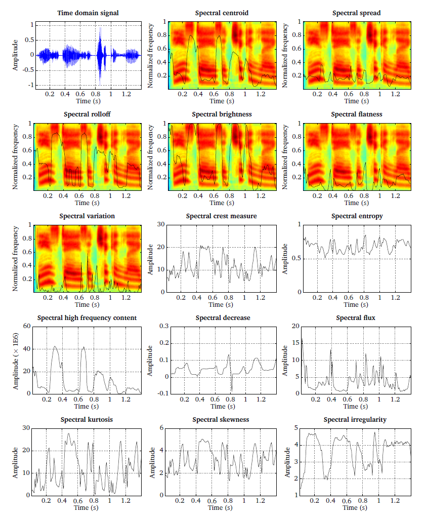
Fig. 27 Speech signal and 14 spectral features that were extracted based on the rate-map representation.
| [Jensen2004] | (1, 2, 3, 4) Jensen, K. and Andersen, T. H. (2004), “Real-time beat estimation using feature extraction,” in Computer Music Modeling and Retrieval, edited by U. K. Wiil, Springer, Berlin– Heidelberg, Lecture Notes in Computer Science, pp. 13–22. |
| [Lerch2012] | (1, 2, 3, 4) Lerch, A. (2012), An Introduction to Audio Content Analysis: Applications in Signal Processing and Music Informatics, John Wiley & Sons, Hoboken, NJ, USA. |
| [Misra2004] | Misra, H., Ikbal, S., Bourlard, H., and Hermansky, H. (2004), “Spectral entropy based feature for robust ASR,” in Proceedings of the IEEE International Conference on Acoustics, Speech and Signal Processing (ICASSP), pp. 193–196. |
| [Peeters2011] | (1, 2, 3, 4, 5, 6, 7, 8) Peeters, G., Giordano, B. L., Susini, P., Misdariis, N., and McAdams, S. (2011), “The timbre toolbox: Extracting audio descriptors from musical signals.” Journal of the Acoustical Society of America 130(5), pp. 2902–2916. |
| [Scheirer1997] | (1, 2) Scheirer, E. and Slaney, M. (1997), “Construction and evaluation of a robust multifeature speech/music discriminator,” in Proceedings of the IEEE International Conference on Acoustics, Speech and Signal Processing (ICASSP), pp. 1331–1334. |
| [Tzanetakis2002] | (1, 2) Tzanetakis, G. and Cook, P. (2002), “Musical genre classification of audio signals,” IEEE Transactions on Audio, Speech, and Language Processing 10(5), pp. 293–302. |