Overview
Framework functionality
The purpose of the Auditory front-end is to extract a subset of common auditory representations from a binaural recording or from a stream of binaural audio data. These representations are to be used later by higher modelling or decision stages. This short description of the role of the Auditory front-end highlights its three fundamental properties:
- The framework operates on a request-based mechanism and extracts the subset of all available representations which has been requested by the user. Most of the available representations are computed from other representations, i.e., they depend on other representations. Because different representations can have a common dependency, the available representations are organised following a “dependency tree”. The framework is built such as to respect this structure and limit redundancy. For example, if a user requests A and B, both depending on a representation C, the software will not compute C twice but will instead reuse it. As will be presented later, to achieve this, the processing is shared among processors. Each processor is responsible for one individual step in the extraction of a given representation. The framework then instantiates only the necessary processors at a given time.
- It can operate on a stream of input data. In other words, the framework can operate on consecutive chunks of input signal, each of arbitrary length, while returning the same output(s) as if the whole signal (i.e., the concatenated chunks) was used as input.
- The user request can be modified at run time, i.e., during the execution of the framework. New representations can be requested, or the parameters of existing representations can be changed in between two blocks of input signal. This mechanism is particularly designed to allow higher stages of the whole Two!Ears framework to provide feedback, requesting adjustments to the computation of auditory representations. In connection to the first point above, when the user requests such a change, the framework will identify where in the dependency tree the requested change starts affecting the processing and will only compute the steps affected.
Getting started
The Auditory front-end was developed entirely using Matlab version 8.3.0.532 (R2014a). It was tested for backward compatibility down to Matlab version 8.0.0.783 (R2012b). The source code, test and demo scripts are all available from the public repository at https://github.com/TWOEARS/auditory-front-end.
All files are divided in three folders, /doc, /src and /test
containing respectively the documentation of the framework, the source code, and
various test scripts. Once Matlab opened, the source code (and if needed the
other folders) should be added to the Matlab path. This can be done by executing
the script startAuditoryFrontEnd in the main folder:
>> startAuditoryFrontEnd
As will be seen in the following subsection, the framework is
request-based: the user places one or more requests, and then informs
the framework that it should perform the processing. Each request
corresponds to a given auditory representation, which is associated with
a short nametag. The command requestList can be used to get a
summary of all supported auditory representations:
>> requestList

  Request name       Label                            Processor
  ------------       -----                            -------------------
  adaptation        Adaptation loop output            adaptationProc
  amsFeatures       Amplitude modulation spectrogram  modulationProc
  autocorrelation   Autocorrelation computation       autocorrelationProc
  crosscorrelation  Crosscorrelation computation      crosscorrelationProc
  filterbank        DRNL output                       drnlProc
  filterbank        Gammatone filterbank output       gammatoneProc
  gabor             Gabor features extraction         gaborProc
  ic                Inter-aural coherence             icProc
  ild               Inter-aural level difference      ildProc
  innerhaircell     Inner hair-cell envelope          ihcProc
  itd               Inter-aural time difference       itdProc
  moc               Medial Olivo-Cochlear feedback    mocProc
  myNewRequest      A description of my new request   templateProc
  offsetMap         Offset map                        offsetMapProc
  offsetStrength    Offset strength                   offsetProc
  onsetMap          Onset map                         onsetMapProc
  onsetStrength     Onset strength                    onsetProc
  pitch             Pitch estimation                  pitchProc
  precedence        Precedence effect                 precedenceProc
  ratemap           Ratemap extraction                ratemapProc
  spectralFeatures  Spectral features                 spectralFeaturesProc
  time              Time domain signal                preProc
A detailed description of the individual processors used to obtain these auditory representations will be given in Available processors.
The implementation of the Auditory front-end is object-oriented, and two objects are needed to extract any representation:
- A data object, in which the input signal, the requested representation, and also the dependent representations that were computed in the process are all stored.
- A manager object which takes care of creating the necessary processors as well as managing the processing.
In the following sections, examples of increasing complexity are given to demonstrate how to create these two objects, and which functionalities they offer.
Computation of an auditory representation
The following sections describe how the Auditory front-end can be used to compute an auditory representation with default parameters of a given input signal. We will start with a simple example, and gradually explain how the user can gain more control over the respective parameters. It is assumed that the entire input signal - for which the auditory representation should be computed - is available. Therefore, this operation is referred to as batch processing. As stated before, the framework is also compatible with chunk-based processing (i.e., when the input signal is acquired continuously over time, but the auditory representation is computed for smaller signal chunks). The chunk-based processing will be explained in a later section.
Using default parameters
As an example, extracting the interaural level difference ’ild’ for a stereo
signal sIn (e.g., obtained from a ’.wav’ file through Matlab´s
wavread) sampled at a frequency fsHz (in Hz) can be done in the
following steps:
1 2 3 4 5 6 7 8 9 | % Instantiation of data and manager objects
dataObj = dataObject(sIn,fsHz);
managerObj = manager(dataObj);
% Request the computation of ILDs
sOut = managerObj.addProcessor('ild');
% Request the processing
managerObj.processSignal;
|
Line 2 and 3 show the instantiation of the two fundamental objects: the
data object and the manager. Note that the data object is always
instantiated first, as the manager needs a data object instance as input
argument to be constructed. The manager instance in line 3 is however an
“empty” instance of the manager class, in the sense that it will not
perform any processing. Hence a processing needs to be requested, as
done in line 6. This particular example will request the computation of
the inter-aural level difference ’ild’. This step is configuring the
manager instance managerObj to perform that type of processing, but
the processing itself is performed at line 9 by calling the
processSignal method of the manager class.
The request of an auditory representation via the addProcessor method of the
manager class on line 6 returns as an output argument a cell array containing a
handle to the requested signal, here named sOut. In the Auditory front-end, signals are
also objects. For example, for the output signal just generated:
>> sOut{1}

ans =

  TimeFrequencySignal with properties:

          cfHz: [1x31 double]
         Label: 'Interaural level difference'
          Name: 'ild'
    Dimensions: 'nSamples x nFilters'
          FsHz: 100
       Channel: 'mono'
          Data: [267x31 circVBufArrayInterface]
This shows the various properties of the signal object sOut. These
properties will be described in detail in the Technical description.
To access the
computed representation, e.g., for further processing, one can create a
copy of the data contained in the signal into a variable, say
myILDs:
>> myILDs = sOut{1}.Data(:);
Note
Note the use of the column operator (:). That is because the property
.Data of signal objects is not a conventional Matlab array and one needs
this syntax to access all the values it stores.
The nature of the .Data property is further described in
Circular buffer.
Input/output signals dimensions
The input signal sIn, for which a given auditory representation
needs be computed, is a simple array. Its first dimension (lines) should
span time. Its first column should correspond to the left channel (or
mono channel, if it is not a stereo signal) and the second column to the
right channel. This is typically the format returned by Matlab´s
embedded functions audioread and wavread.
The input signal can be either mono or stereo/binaural. The framework can operate on both. However, some representations, such as the as the ILD as requested in the previous example, are based on a comparison between the left and the right ear signals. If a mono signal was provided instead of a binaural signal, the request of computing the ILD representation would produce the following warning and the request would not be computed:
Warning: Cannot instantiate a binaural processor with a mono input signal!
> In manager>manager.addProcessor at 1127
The dimensions of the output signal from the addProcessor method
will depend on the representation requested. In the previous example,
the ’ild’ request returns a single output for a stereo input.
However, when the request is based on a single channel and the input is
stereo, the processing will be performed for left and right channel, and
both left and right outputs are returned. In such cases, the output from
the method addProcessor will be a cell array of dimensions 1 x 2
containing output signals for the left channel (first column) and right
channel (second column). For example, the returned sOut could take
the form:
>> sOut

sOut =

    [1x1 TimeFrequencySignal]    [1x1 TimeFrequencySignal]
The left-channel output can be accessed using sOut{1}, and
similarly, sOut{2} for the right-channel output.
Change parameters used for computation
For the requested representation
Each individual processors that is supported by the Auditory front-end can be controlled
by a set of parameters. Each parameter can be accessed by a unique
nametag and has a default value. A summary of all parameter names and
default values for the individual processors can be listed by the
command parameterHelper:
>> parameterHelper

Parameter handling in the TWO!EARS Auditory Front-End
-------------------------------------------------
The extraction of various auditory representations performed by the TWO!EARS Auditory Front-End software involves many parameters. Each parameter is given a unique name and a default value. When placing a request for TWO!EARS auditory front-end processing that uses one or more non-default parameters, a specific structure of non-default parameters needs to be provided as input. Such structure can be generated from |genParStruct|, using pairs of parameter name and chosen value as inputs.

Parameters names for each processor are listed below:
            Amplitude modulation|
            Auto-correlation|
            Cross-correlation|
            DRNL filterbank|
            Gabor features extractor|
            Gammatone filterbank|
            IC Extractor|
            ILD Extractor|
            ITD Extractor|
            Medial Olivo-Cochlear feedback processor|
            Inner hair-cell envelope extraction|
            Neural adaptation model|
            Offset detection|
            Offset mapping|
            Onset detection|
            Onset mapping|
            Pitch|
            Pre-processing stage|
            Precedence effect|
            Ratemap|
            Spectral features|
            Plotting parameters|
Each element in the list is a hyperlink, which will reveal the list of parameters for a given element, e.g.,
Inter-aural Level Difference Extractor parameters::

  Name            Default   Description
  ----            -------   -----------
  ild_wname       'hann'    Window name
  ild_wSizeSec    0.02      Window duration (s)
  ild_hSizeSec    0.01      Window step size (s)
It can be seen that the ILD processor can be controlled by three parameters,
namely ild_wname, ild_wSizeSec and ild_hSizeSec. A particular
parameter can be changed by creating a parameter structure which contains the
parameter name (nametags) and the corresponding value. The function
genParStruct can be used to create such a parameter structure. For
instance:
>> parameters = genParStruct('ild_wSizeSec',0.04,'ild_hSizeSec',0.02)

parameters =

  Parameters with properties:

    ild_hSizeSec: 0.0200
    ild_wSizeSec: 0.0400
will generate a suitable parameter structure parameters to request the
computation of ILD with a window duration of 40 ms and a step size of 20 ms.
This parameter structure is then passed as a second input argument in the
addProcessor method of a manager object. The previous example can be
rewritten considering the change in parameter values as follows:
% Instantiation of data and manager objects
dataObj = dataObject(sIn,fsHz);
managerObj = manager(dataObj);

% Non-default parameter values
parameters = genParStruct('ild_wSizeSec',0.04,'ild_hSizeSec',0.02);

% Place a request for the computation of ILDs
sOut = managerObj.addProcessor('ild',parameters);

% Perform processing
managerObj.processSignal;
For a dependency of the request
The previous example showed that the processor extracting ILDs was accepting three parameters. However, the representation it returns, the ILDs, will depend on more than these three parameters. For instance, it includes a certain number of frequency channels, but there is no parameter to control these in the ILD processor. That is because such parameters are from other processors that were used in intermediate steps to obtain the ILD. Controlling these parameters therefore requires knowledge of the individual steps in the processing.
Most auditory representations will depend on another representation,
itself being derived from yet another one. Thus, there is a chain of
dependencies between different representations, and multiple
processing stages will be required to compute a particular output. The
list of dependencies for a given processor can be visualised using the
function Processor.getDependencyList(’processorName’), e.g.
>> Processor.getDependencyList('ildProc')

ans =

    'innerhaircell'    'filterbank'    'time'
shows that the ILD depends on the inner hair-cell representation
(’innerhaircell’), which itself is obtained from the output of a gammatone
filter bank (’filterbank’). The filter bank is derived from the time-domain
signal, which itself has no further dependency as it is directly derived from
the input signal.
When placing a request to the manager, the user can also request a change in
parameters of any of the request’s dependencies. For example, the number of
frequency channels in the ILD representation is a property of the filter bank,
controlled by the parameter ’fb_nChannels’. (which name can be found using
parameterHelper.m). This parameter can also be requested to have a
non-default value, although it is not a parameter of the processor in charge of
computing the ILD. This is done in the same way as previously shown:
% Non-default parameter values
parameters = genParStruct('fb_nChannels',16);

% Place a request for the computation of ILDs
sOut = managerObj.addProcessor('ild',parameters);

% Perform processing
managerObj.processSignal;
The resulting ILD representation stored in sOut{1} will be based on 16
channels, instead of 31.
Compute multiple auditory representations
Place multiple requests
Multiple requests are supported in the framework, and can be carried
out by consecutive calls to the addProcessor method of an instance
of the manager with a single request argument. It is also possible to
have a single call to the addProcessor method with a cell array of
requests, e.g.:
% Place a request for the computation of ILDs AND autocorrelation
[sOut1 sOut2] = managerObj.addProcessor({'ild','autocorrelation'})
This way, the manager set up in the previous example will extract an ILD and
an auto-correlation representation, and provide handles to the three signals, in
sOut1{1} for the ILD (it is a mono representation), sOut2{1} and
sOut2{2} for the autocorrelations of respectively left and right channels.
To use non-default parameter values, three syntax are possible:
If there are several requests, but all use the same set of parameter values
p:managerObj.addProcessor({'name1', .. ,'nameN'},p)
If there is only one request (
name), but with different sets of parameter values (p1,...,pN), e.g., for investigating the influence of a given parametermanagerObj.addProcessor('name',{p1, .. ,pN})
If there are several requests and some, or all, of them use a different set of parameter values, then it is necessary to have a set of parameter (
p1,...,pN) for each request (possibly by duplicating the common ones) and place them in a cell array as follows:managerObj.addProcessor({'name1', .. ,'nameN'},{p1, .. ,pN})
Note that in the two examples above, no output is specified for the
addProcessor method, but the representations will be computed
nonetheless. The output of addProcessor is there for convenience and
the following subsection will explain how to get a hang on the computed
signals without an explicit output from addProcessor.
Requests can also be placed directly as optional arguments in the manager constructor, e.g., to reproduce the previous script example:
% Instantiation of data and manager objects
dataObj = dataObject(sIn,fsHz);
managerObj = manager(dataObj,{'ild','autocorrelation'});
The three possibilities described above can also be used in this syntax form.
Computing the signals
This is done in the exact same way as for a single request, by calling
the processSignal method of the manager:
% Perform processing
managerObj.processSignal;
Access internal signals
The optional output of the addProcessor method is provided for
convenience. It is actually a pointer (or handle, in Matlab´s terms) to
the actual signal object which is hosted by the data object on which the
manager is based. Once the processing is carried out, the properties of
the data object can be inspected:
>> dataObj

dataObj =

  dataObject with properties:

   bufferSize_s: 10
       isStereo: 1
            ild: {[1x1 TimeFrequencySignal]}
  innerhaircell: {[1x1 TimeFrequencySignal]  [1x1 TimeFrequencySignal]}
          input: {[1x1 TimeDomainSignal]  [1x1 TimeDomainSignal]}
           time: {[1x1 TimeDomainSignal]  [1x1 TimeDomainSignal]}
     filterbank: {[1x1 TimeFrequencySignal]  [1x1 TimeFrequencySignal]}
autocorrelation: {[1x1 CorrelationSignal]  [1x1 CorrelationSignal]}
Apart from the properties bufferSize_s and isStereo which are inherent
properties of the data object (and discussed later in the
Technical description), the remaining properties each correspond to
one of the representations computed to achieve the user’s request(s). They are
each arranged in cell arrays, with first column being the left, or mono channel,
and the second column the right channel. For instance, to get a handle
sGammaR to the right channel of the gammatone filter bank output, type:
>> sGammaR = dataObj.filterbank{2}

sGammaR =

  TimeFrequencySignal with properties:

      cfHz: [1x31 double]
     Label: 'Gammatone filterbank output'
      Name: 'filterbank'
Dimensions: 'nSamples x nFilters'
      FsHz: 44100
   Channel: 'right'
      Data: [118299x31 circVBufArrayInterface]
How to plot the result
Plotting auditory representations is made very easy in the Auditory front-end. As explained
before, each representation that was computed during a session is stored as a
signal object, which each are individual properties of the data object. Signal
objects of each type have a plot method. Called without any input
arguments, signal.plot will adequately plot the representation stored in
signal in a new figure, and returns as output a handle to said figure. The
plotting method for all signals can accept at least one optional argument, which
is a handle to an already existing figure or subplot in a figure. This way the
representation can be included in an existing plot. A second optional argument
is a structure of non-default plot parameters. The parameterHelper script
also lists plotting options, and they can be modified in the same way as
processor parameters, via the script genParStruct. These concepts can be
summed up in the following example lines, that follows right after the demo code
from the previous subsection:
1 2 3 4 5 6 7 8 9 10 11 12 13 14 15 16 17 18 19 20 21 | % Request the processing
managerObj.processSignal;
% Plot the ILDs in a separate figure
sOut{1}.plot;
% Create an empty figure with subplots
figure;
h1 = subplot(2,2,1);
h2 = subplot(2,2,2);
h3 = subplot(2,2,3);
h4 = subplot(2,2,4);
% Change plotting options to remove colorbar and reduce title size
p = genParStruct('bColorbar',0,'fsize_title',12);
% Plot additional representations
dataObj.innerhaircell{1}.plot(h1,p);
dataObj.innerhaircell{2}.plot(h2,p);
dataObj.filterbank{1}.plot(h3,p);
dataObj.filterbank{2}.plot(h4,p);
|
This script will produce the two figure windows displayed in Fig. 3. Line 22 of the script creates the window “Figure 1”, while lines 35 to 38 populate the window “Figure 2” which was created earlier (in lines 25 to 29).
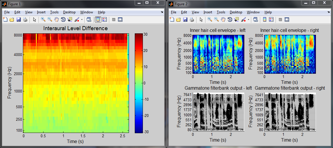
Fig. 3 The two example figures generated by the demo script.
Chunk-based processing
As mentioned in the previous section, the framework is designed to be compatible with chunk-based processing. As opposed to “batch processing”, where the entire input signal is known a priori, this means working with consecutive chunks of input signals of arbitrary size. In practice the chunk size will often be the same from one chunk to another. However, this is not a requirement here, and the framework can accept input chunks of varying size.
The main constraint behind working with an input that is segmented into chunks is that the returned output should be exactly the same as if the whole input signal (i.e., the concatenated chunks) was used as input. In other terms, the transition from one chunk to the next needs to be taken into account in the processing. For example, concatenating the outputs obtained from a simple filter applied separately to two consecutive chunks will not provide the same output as if the concatenated chunks were used as input. To obtain the same output, one should for example use methods such as overlap-add or overlap-save. This is not trivial, particularly in the context of the Auditory front-end where more complex operations than simple filtering are involved. A general description of the method used to ensure chunk-based processing is given in processChunk method and chunk-based compatibility.
Handling segmented input in practice is done mostly the same way as for a whole
input signal. The available demo script DEMO_ChunkBased.m provides an
example of chunk-based processing by simulating a chunk-based acquisition of the
input signal with variable chunk size and computing the corresponding ILDs.
In this script, one can note the two differences in using the Auditory front-end in a chunk-based scenario, in comparison to a batch scenario:
21 22 23 | % Instantiation of data and manager objects
dataObj = dataObject([],fsHz,10,2);
managerObj = manager(dataObj);
|
Because the signal is not known before the processing is carried out, the data
object cannot be initialised from the input signal. Hence, as is seen on line
22, one needs to instantiate an empty data object, by leaving the first input
argument blank. The sampling frequency is still necessary however. The third
argument (here set to 10) is a global signal buffer size in seconds. Because
in an online scenario, the framework could be operating over a long period of
time, internal representations cannot be stored over the whole duration and are
instead kept for the duration mentioned there. The last argument (2)
indicates the number of channel that the framework should expect from the input
(a mono input would have been indicated by 1). Again, it is necessary to
know the number of channels in the input signal, to instantiate the necessary
objects in the data object and the manager.
43 44 | % Request the processing of the chunk
managerObj.processChunk(sIn(chunkStart:chunkStop,:),1);
|
The processing is carried out on line 44 by calling the processChunk method
of the manager. This method takes as input argument the new chunk of input
signal. The additional argument, 1, indicates that the results should be
appended to the internal representations already computed. This can be set to
0 in cases where keeping track of the output for the previous chunks is
unnecessary, for instance if the output of the current chunk is used by a
higher-level function. The difference with the processSignal method is
important. Although processSignal actually calls internally
processChunk, it also resets internal states of the framework (what ensures
continuity between chunks) before processing.
The script DEMO_ChunkBased.m will also compute the offline result and will
plot the difference in output for the two computations. This plot is shown in
Fig. 4. Note the magnitude on the order of
\(10^{-15}\), which is in the range of Matlab numerical precision,
suggesting that the representations computed online or offline are the same up
to some round-off errors.
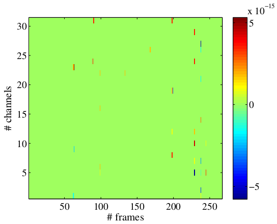
Fig. 4 Difference in ILDs obtained with online and offline processing
Feedback inclusion
A key concept of the Auditory front-end is its ability to respond to feedback from the user or from external, higher stage models. Conceptually, feedback at the stage of auditory feature extraction is realised by allowing changes in parameters and/or changes in which features are extracted at run time, i.e., in between two chunks of input signal in a chunk-based processing scenario.
In practice, three types of feedback can be identified: - A new request is placed - One or more parameters of an existing request is changed - A processor has become obsolete and is deleted
Placing a new request
Placing a new request at run time, i.e., online, is done exactly is it is done
offline, by calling the
.addProcessor method of an existing manager instance.
Modifying a processor parameter
Warning
Some parameters are blacklisted for modifications as they would imply a change in dimension in the output signal of the processor. If you need to perform this change anyway, consider placing a new request instead of modifying an existing one.
Modifying a processor parameter can be done by calling the modifyParameter
method of that processor in between two calls to the processChunk of the
manager instance.
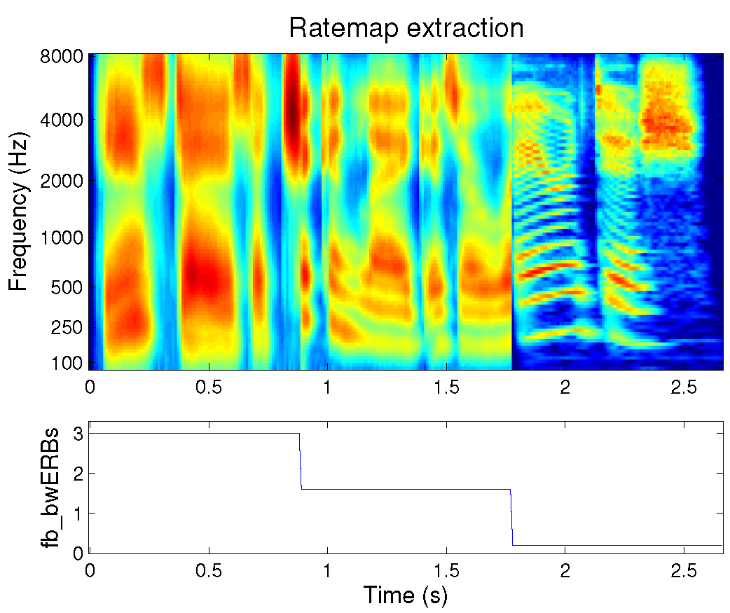
Fig. 5 Sharpening the frequency selectivity of the ear by means of feedback
Fig. 5 illustrates feedback capability of the Auditory front-end.
This is a rate-map representation of a speech signal that is extracted online.
The bandwidth of auditory filters, controlled by the parameter fb_bwERBs in
the original request was set to 3 ERBs, an abnormally large value in
comparison to a normal-hearing frequency selectivity. Throughout the
processing, the bandwidth is reduced to 1.5 ERBs by calling:
mObj.Processors{2}.modifyParameter('fb_bwERBs',1.5);
in between two calls to the processChunk method of the manager mObj, at
around 0.9s. Here, mObj.Processors{2} points to the auditory filterbank
processor, an instance of a gammatone processor. The bandwidth is later (at
1.75s) reduced even further (to about 0.25). Fig. 5
illustrates how narrower auditory filters will reveal the harmonic structure of
speech.
Note
If a processor is modified in response to feedback, subsequent processors need to reset themselves, in order not to carry on incorrect internal states. This is done automatically inside the framework. For example, in the figure above, internal filters of the inner hair-cell envelope extraction and the ratemap computation are reset accordingly when the bandwidth parameter is changed
Deleting a processor
Deleting a processor is simply done by calling its remove method. Like for
parameter modifications, this affects subsequent processors, as they will also
become obsolete. Hence they will also be automatically deleted.
Deleting processors will leave empty entries in the manager.Processors cell
array. To clean up the list of processor, call the cleanup() method of your
manager instance.
List of commands
This section sums up the commands that could be relevant to a standard user of the Auditory front-end. It does not describe each action extensively, nor does it give a full list of corresponding parameters. A more detailed description can be obtained through calling the help script of a given method from Matlab´s command window. Note that one can get help on a specific method of a given class. For example
>> help manager.processChunk
will return help related to the processChunk method of the manager class.
The following aims at being concise, hence optional inputs are marked as
“...” and can be reviewed from the specific method help.
Signal objects sObj
sObj.Data(:) |
Returns all the data in the signal |
sObj.Data(n1:n2) |
Returns the data in the time interval [n1,n2] (samples) |
sObj.findProcessor(mObj) |
Finds processor that computed the signal |
sObj.getParameters(mObj) |
Parameter summary for that signal |
sObj.getSignalBlock(T,...) |
Returns last T seconds of the signal |
sObj.play |
Plays back the signal (time-domain signals only) |
sObj.plot(...) |
Plots the signal |
Data objects dObj
dataObject(s,fs,bufSize,nChannels) |
Constructor |
dObj.addSignal(sObj) |
Adds a signal object |
dObj.clearData |
Clears all signals in dObj |
dObj.getParameterSummary(mObj) |
Lists parameter used for each signal |
dObj.play |
Plays back the containing audio signal |
Processors pObj
pObj.LowerDependencies |
List of processors pObj depends on |
pObj.UpperDependencies |
List of processors depending on pObj |
pObj.getCurrentParameters |
Parameter summary for that processor |
pObj.getDependentParameter(parName) |
Value of a parameter from pObj or its dependencies |
pObj.hasParameters(parStruct) |
True if pObj used the exact values in parStruct |
pObj.Input |
Handle to input signal object |
pObj.Output |
Handle to output signal object |
pObj.modifyParameter |
Change a parameter value |
pObj.remove |
Removes a processor (and its subsequent processors) |
Manager mObj
manager(dObj) |
Constructor |
manager(dObj,name,param) |
Constructor with initial request |
mObj.addProcessor(name,param) |
Adds a processor (including eventual dependencies) |
mObj.Data |
Handle to the associated data object |
mObj.processChunk(input,...) |
Process a new chunk |
mObj.Processors |
Lists instantiated processors |
mObj.processSignal |
Process a signal offline |
mObj.reset |
Resets all processors |
mObj.cleanup |
Cleans up the list of processors |
Acknowledgement
The Auditory front-end includes the following contributions from publicly available Matlab toolboxes or classes: